오늘도 역시 action Recognition 과 관련된 논문입니다.
skeleton based model일텐데 한번 봅시다.
Abstract
skeleton-based action recognition에서 GCN은 human body skeleton을 spatiotemporal graphs로 model 하죠. GCNs는 remarkable performance를 달성했고요. 그러나 existing GCN-based methods는 graph의 topology를 manually하게 set하죠. 그리고 all layers와 input samples에 걸쳐 fixed 되죠. 이것은 action recognition task에서 hierarchical GCN과 diverse samples을 위한 optimal이 아닙니다. 게다가, skeleton data의 second-order information ( bone의 lengths and directions ) 는 action recognition에 대해 naturally 더 informative하고 discriminative하죠. existing method에서는 거의 사용되지 않았고요. 이 연구에서, 저자들은 새로운 two-stream adaptive graph convolutional network ( 2s-AGCN )을 제안하는데 skeleton based action recognition을 위한 model이죠. graph의 topology는 uniformly 나 individually BP algorithm에 의해 end-to-end로 학습될 수 있죠. 이 data-driven method는 graph construction을 위한 model의 flexibility를 증가시키죠. 그리고 varous data samples에 adapt하는 more generality를 야기하고요. 게다가 two-stream framework는 first-order와 second-order information을 동시에 model 하기 위해 제안됩니다. 이는 recognition accuracy에 대해 notable improvemnet를 보여주죠.
Introduction
Action recognition methods는 skeleton data 에 기반하고 dynamic circumstane 와 complicated background에 strong adaptability 때문에 considerable attenion 을 attracted하고 investigated 되어왔죠. Conventional deep-learning-based methods는 skeleton을 joint-coordinate vectors 의 sequence나 prediction을 generate하는 RNNs 나 CNNs 입력으로 주어지는 pseudo-image 로 manually structure 합니다. 그러나, sklelton data를 vector sequence나 2D grid 로 representing하는 것은 correlated joints 간의 dependency 를 완전히 express할 수 없죠. skeleton은 joints를 vertexes로 하고 human body에서 connections를 edges로 가진 non-Euclidean space에서 graph로써 structured 되죠. 이전 methods는 skeleton data의 graph structure을 사용할수 없죠. arbitray forms를 가진 skeleton으로 generalize하기 어렵고요. 최근 GCNs는 image로 부터 graph에 이르기 까지 convolution을 genralize합니다. GCNs는 많은 applications에 성공적으로 adopted 되었죠. skeleton based action reconitoin task에 대해 Yan은 GCNs를 skeleton data를 model 하는데 처음 적용했습니다. 그들은 joint의 natural connections에 기반한 spatial graph를 construct했죠. 그리고 consecutive frames에서 corresponding joints 간에 temporal edges를 추가했습니다. distance-based sampling function은 graph convolutional layer를 constructing 하기 위해 제안되었고, final spatiotemporal graph convolutional network( ST-GCN )을 build하는 basic module로써 사용되죠.
그러나, ST-GCN에서 graph construction의 process에는 3 가지 결점이 있는데요; (1) ST-GCN에서 사용된 skeleton graph는 heuristically predefined 되었죠. 그리고 human body의 physical structure 만이 represents 됩니다. 따라서 action recognition task에 대해 optimal을 보장하지 못합니다. 가령, two hands 간의 relationship은 "clapping" 과 "reading" 과 같이 recognizing classes를 위해서는 중요하죠. 그러나 ST-GCN은 two hands 간의 dependency를 capture하기 어렵죠. 왜냐하면 두 손은 predefined human-body-based graphs에서 서로 멀리 떨어져 있기 때문이죠. (2) GCNs의 structure는 hierarchical 합니다. different layers는 multilevel semantic information을 contain하죠. 그러나, ST-GCN에 applied된 graph의 topology는 all layers에 걸쳐 fixed되죠. 이는 모든 layers에서 contained 된 multilevel semantic information을 model하는 capacity와 flexibility를 lack 하게 하고요. (3) One fixed graph structure는 different acion classes에 optimal 하지 않을 수 있죠. "wiping face"와 "touching head"와 같은 classes에 대해, hands와 head 간의 connection은 stronger해야하죠. 그러나 "jumping up" 이나 "sitting down"과 같은 classes에서는 그러면 안되고요. 이런 사실은 graph structure가 data dependent해야 하고 ST-GCN에서는 지원하지 않는다는 것을 암시하죠.
이 문제를 해결하기 위해, 새로운 adaptive graph convolutional network가 이 연구에서 제안되었는데요. model의 convolutional parameters를 가지고 동시에 trained되고 updated 되는 두 종류의 graphs를 parameterized합니다. 하나의 type은 global graph인데요. all data에 대해 common pattern을 represents하죠. 다른 type은 indiviual graph인데요. 각 data에 대해 unique pattern을 represents하죠. graphs의 two types 모두 different layers에 대해 individually 하게 optimized됩니다. model의 hierarchical structure를 더 잘 fit 할 수 있죠. data-driven method는 graph construction에 대한 model의 flexibility를 증가시키죠. 그리고 various data samples에 adapt하는 more generality를 야기합니다.
ST-GCN에서 Another notable problem은 vertex에 attached된 feature vector는 오직 2D 나 3D joints의 coordinates를 contains하죠. skeleton data의 first-order information으로써 여겨질 수 있죠. 그러나 second-order information은 두 joints 간의 bones의 feature를 represents하는데, 사용되지 않죠. Typically, bones의 lengths와 directions는 action recognition에 대해 more informative 하고 discriminative 하죠. skeleton data의 second-order information을 사용하기 위해, bones의 lengths와 directions는 source joint로부터 target joint로 vector pointing로써 formulated 하죠. first-order information과 유사하게, vector는 action label을 predict하는 adaptive graph convolutional network의 입력으로 던져줍니다. 게다가 , two-stream framework은 first-order와 second-order infromation 을 fuse하기 위해 제안되고요.
proposed model의 우월성을 증명하기 위해, 2s-AGCN은 NTU-RGBD 와 kinetics-Skeleton에서 실험이 진행되었죠. 모두에서 SOTA 성능을 달성했고요
main contributions는 3가지 입니다: (1) adaptive graph convolutional network는 different GCN layers와 skeleton samles에 대한 graph의 topology를 end-to-end 방법으로 학습하기 위해 제안됩니다. 이는 action recognition task와 hirarchical structure에 better suit하죠. (2) skeleton data의 second-order information 은 explicitly하게 formulated되죠. 그리고 two-stream framework을 사용해 first-order information과 결합되죠. 이는 성능에 좋은 영향을 미치고요. (3) skeleton-based action recognition을 위한 두 가지 large-scale datasets에서 SOTA 성능을 달성했죠.
Related work
Skeleton-based action recognition
skeleton-based action recognition을 위한 conventional methods는 대게 human body를 model하는 handcrafted features를 design하죠. 그러나, 이 handcrafted-feature-based methods의 performance는 satisfactory하지 않죠. 동시에 all factors를 consider 할 수 없기 때문이죠. deep learning의 development에 힘입어, data-driven methods는 mainstream methods가 되었죠. 가장 많이 사용되는 model은 RNNs와 CNNs 이고요. RNN-based methods는 skeleton data를 human body joint를 represents하는 coordinate vectors의 sequence로 model 하죠. CNN-based methods는 skeleton data를 pseudo-image로 model하는데 designed된 transformation rules에 기반하죠. CNN-based methods는 RNN-based methods 보다 more popular합니다. 왜냐하면 CNNs 가 better parallelizability를 가지고 있고 RNNs보다 train하기 쉽기 때문이죠.
그러나, RNNs와 CNNs는 skeleton data의 structure를 fully represent 하는 데 실패하죠. skeleton data가 vector sequence 나 2D grid 라기 보다 graphs의 형태로 embedded 되기 때문이죠. 최근 Yan은 ST-GCN을 제안하죠. skeleton data를 graph structure로 directly하게 model하죠. 이는 handcrafted part assignment나 traversal rules를 designing 할 need를 제거하죠. 따라서 이전 방법들보다 더 좋은 performance를 달성합니다.
Graph convolutional neural networks
graph convolution에 관한 많은 연구가 있습니다. 그리고 constructing GCNs의 principle은 두 가지의 stream이 있죠. spatial perspective와 spectral perspective 가 있죠. Spatial perspective methods는 graph vertexes와 그들의 neighbors에 대해 convolution filters를 직접 수행하죠. 이는 disigned rules에 기반해 normalized 하고 extracted 되죠. 반면, spetral perspective methods는 Laplace matrices의 eigenvalues와 eigenvectors 를 사용하죠. 이런 방법들은 graph Fourier transform 의 도움을 받아, frequency domain에서 graph convolution을 수행합니다. 이는 각 convolutional step에서 graphs로부터 connected regions를 locally하게 extract 할 필요가 없죠. 이 연구는 spatial perspective methods를 따르죠.
Graph Convolutional Networks
Graph construction
한 frame에서 raw skeleton data는 always vector의 sequece로써 주어지죠. 각 vector는 corresponding human joint의 2D 나 3D coordinates로 represents 되죠. complete action은 different samples에 대해 different lengths 가진 multiple frames를 포함하죠. 저자들은 spatiotemporal graph를 사용하는데 이는 spatial and temporal dimesions 에 따라 joints 중에 structured information을 model하죠. graph의 structure는 ST-GCN의 work을 따르죠. Fig 1의 left sketch는 constructed spatiotemporal skeleton grahp의 example을 나타내죠. 여기서 joints는 vertexes로 나타나고 human body에서 natrual connections는 spatial edges로 나타나죠.( Fig 1에서는 orange line 입니다. )

temporal dimension에 대해, 두 개의 adjacnet frames 간의 corresponding joints는 temporal edges로 연결되죠 ( Fig 1에서 blue line이 되겠죠 ). 각 joint의 coordinate vector는 corresponding vertex의 attribute로써 set됩니다.
Graph convolution
위에서 정의한데로 graph 가 주어지면, spatiotemporal graph convolution operation의 multiple layers 가 high-level features를 extract하기 위해 applied되죠. global average pooling layer 와 softmax classifier가 extracted features에 기반해 action categories를 predict하기 위해 사용됩니다.
spatial dimension에서, vertex v_i에 대한 graph convolution operation는 아래와 같이 공식화 되죠.

f는 feature map을 denotes합니다. v 는 graph의 vertex를 표기하고요. B_i는 v_i에 대한 convolution 의 sampling area를 표기하는데, 이는 target vertex( v_i )의 1-distance neighbor vertexes( v_j ) 로써 정의되죠. w 는 original convolution operation에서와 유사한 weighting function이고 주어진 input에 기반해 weight vector를 provide하죠. convolution의 weight vectors 수는 fixed되어있는 반면 B_i에서 vertexes의 수는 varied 된다는 것을 강조합니다. unique weight vector를 가진 각 vertex를 map하기 위해 , mapping function l_i는 ST-GCN에서 specially하게 desinged 되었죠. Fig 1의 right sketch이고 strategy를 보여주죠. 여기서 x 는 skeleton의 gravity의 center를 represent하죠. B_i 는 curve로 enclosed된 area이고요. 상세히 말하면, strategy는 kernel size를 3으로 set하고 B_i를 3 개의 subset으로 나누죠: S_i1은 vertex 그자체인데요, ( Fig 1의 오른쪽 에서 red cirecle입니다 ); S_i2는 centripetal subset이고 gravity의 center에 더 가까운 neighboring vertexs를 포함하고 그림에서는 green circle이죠; S_i3은 centrifugal subset으로 gravity 의 center로부터 좀 더 먼 neighboring vertexs를 contains 하고 blue circle이죠. Z_ij는 S_ik의 cardinality를 표기하는데 v_j를 포함하죠. 이는 each subset의 contribution을 balance하는 것을 목적으로 합니다.
Impelmentation
spatial dimension에서 graph convolution의 implementation은 직관적이지 않죠. 구체적으로 network의 feature map은 C x T x N tensor 이죠. 여기서 N은 vertex의 number를 표기하고, T는 temporal length를 , C는 channels의 number를 표기하죠. ST-GCN을 implement하기 위해, Eq 1이 아래 식으로 transformed 되죠.

여기서 K_v는 spatial dimension의 kernel size를 표기하죠. 위에 designed된 partiion strategy에서, K_v는 3으로 set되죠.

이고 barA_k는 N x N adjacency matrix와 유사하죠. elements bar A^ij_k는 vertex v_j 가 vertex v_i의 subset S_ik에 존재하는 지를 나타냅니다. 이는 corresponding weight vector에 대해 f_in 으로부터 particular subset에서 connected vertexes를 extract하는데 사용되죠.

lamda ^ii_k 는 normalized diagonal matrix입니다. alpha는 0.001로 set하고 empty row를 피하기 위함이죠. W_k는 1x1 convolution operation의 C_out x C_in x 1 x 1 weight vector이고 Eq1에서 weighting function w를 represent하죠. M_k는 N x N attention map이고 each vertex의 importance를 나타냅니다. double circle은 dot product를 나타내고요.
temporal dimension에 대해, 각 vertex에 대해 neighbors의 수가 2로 fixed 되어 있기 때문에 ( 두 개의 consecutive frames에서 corresponding joints를 나타내니까요 ), classical convolution operation과 유사하게 graph convolution이 직관적으로 수행되죠. 구체적으로, 저자들은 K_t x 1 convolution을 위에서 계산된 output feature map에 대해 perform 하죠. 여기서 K_t 는 temporal dimension의 kernel size이죠.
Two-stream adaptive graph convolutional network
이 section에서, 저자들은 2s-AGCN의 components를 자세히 설명합니다.
Adaptive graph convolutional layer
skeleton data를 위한 spatiotemporal graph convoltution 은 predefined graph에 기반해 calculated되죠. 이는 처음에 설명했던것처럼 best choice가 아닐 수 있고요. 이 문제를 해결하기 위해, 저자들은 adaptive graph convolutional layer를 제안합니다. 이는 graph의 topology를 만드는데, end-to-end learining manner에서 network의 other paramters를 가지고 함께 optimized 되죠. graph는 different layers와 samples에 대해 unique하죠. 이는 model의 flexibility를 greatly increase하고요. 그러는 동안에, 이는 residual branch로 designed되고, original model의 stability를 보장하죠.
자세히, Eq2 를 따라, graph의 topoloy는 adjacency marix와 mask에 의해 결정되죠. 가령, A_k와 M_k 각각 말이죠. A_k는 두 개의 vertex간에 connections가 있는 지를 결정하고, M_k는 connections의 strength를 결정합니다. graph strcutre를 adaptive하게 하기 위해, Eq 2를 아래와 같이 바꿉니다.

주요한 difference는 graph의 adjacency matrix에 있는데요. 3 개의 parts로 나눠지고 각각 A_k, B_k, C_k입니다. A_k는 original marmalized N x N adjacency matrix A_k 이고 Eq 2에서와 동일합니다. 이는 human body의 physical sturcture을 represents하죠.
B_k 역시 N x N adjacency matrix이죠. A_k 와 대조되는 점은, B_k의 elements는 training process에서 other parameters와 함께 optimized되고 parameterized되죠. B_k의 value에 대한 constraints는 없습니다. 이것은 graph가 training data에 따라 completely learned 됨을 의미하죠. 이 data-driven manner로, model은 recognition task에 fully targeted 되고 different layers에 contained된 different information에 대해 more individualized 되는 graph를 learn할 수 있죠. matrix에서 element는 arbitrary value가 될 수 있습니다. 이는 Eq2에서 M_k에 의해 수행되는 attention mechanism의 역할을 할 수 있죠. 그러나, original attention matrix M_k는 A_k에 dot multiplied 되죠. 이는 A_k에서 elements 중 하나가 0이라면, M_k의 value에 상관없이 항상 0이 됨을 의미하죠. 따라서, original physical graph에 존재하지 않는 new connections를 만들 수 없습니다. 이런 관점에서, B_k는 M_k보다 더 flexible 하죠.
C_k는 data-dependent graph인데요. 각 sample에 대해 unique graph를 learn하죠. 두 개의 vetexs 간의 connection이 있는지, connection이 얼마나 strong 한지를 결정하기 위해, 저자들은 two vertexs의 similarity를 계산하는 normalized embedded Gausian function을 apply하고 식은 아래와 같습니다.
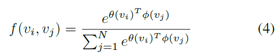
N은 vertexes의 number를 뜻합니다. 저자들은 dot product를 사용하는데, embedding space에서 two vertexs의 similarity를 measure하죠. 구체적으로, size가 C_in x T x N인 input feature map f_in이 주어지면, 저자들은 먼저 두 개의 embedding functions를 가지고 C_e x T x N로 embed합니다. 예를 들면, theta 와 pi 죠. 여기서, extensive experiments를 통해, 저자들은 1 x 1 convolutional layer를 rearranged 하고 N x C_eT matrix와 C_eT x N matrix으로 reshaped 하는 function을 고릅니다. 그리고나면 matrix들은 N x N similarity matrix C_k를 얻기 위해 multiplied 되죠. 여기서 C^ij_k element는 vertex v_i 와 v_j 의 similarity를 represents 하죠. matrxi의 value는 0-1로 normalized 되죠. 이는 두 개의 vertexes의 soft edge로써 사용되고요. normalized Gaussian은 softmax operation이 포함되어 있기 때문에, C_k를 Eq4에 기반해 계산할 수 있죠. 이를 식으로 나타내면 아래와 같고요.
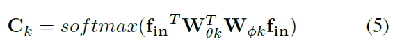
W_theta와 W_pi는 embedding functions theta와 pi의 parameters 이죠.
A_k를 B_k 나 C_k로 직접 대체하는 대신에, 저자들은 그들을 A_k에 더하죠. B_k의 value와 theta와 pi의 parameters는 -으로 initialized됩니다. 이런 방식으로, original performance의 감소 없이 model의 flexibility를 강화할 수 있죠.
adaptive graph convolution layer의 overall architecture는 Fig2. 에서 볼 수 있는데요.
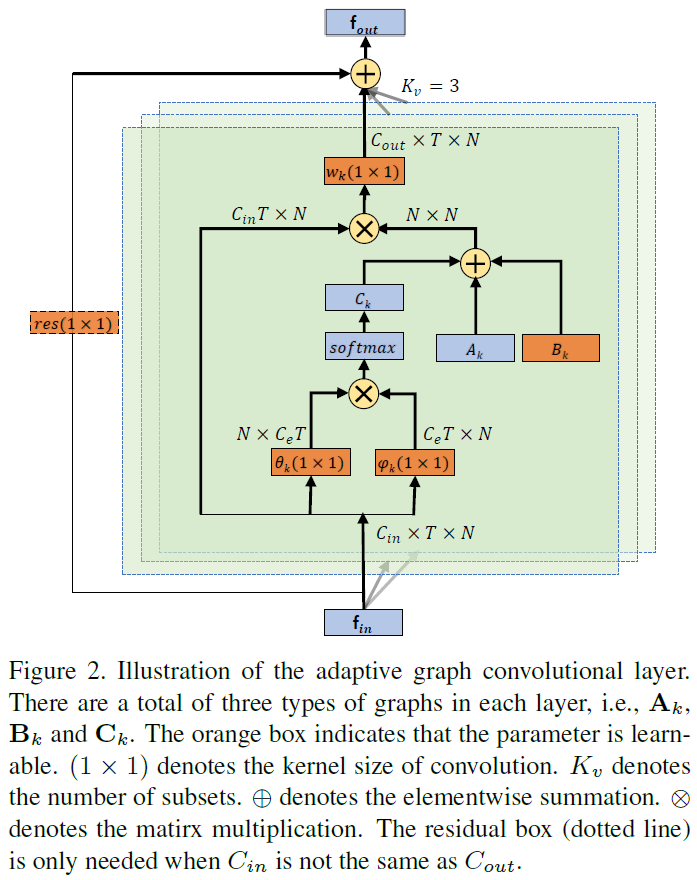
A_k, B_k, C_k 가 도입된것을 제외하고, convolution의 kernel size ( K_v )는 전과 같이 set하죠. w_k는 Eq 1에서 설명한 weighting function입니다. w_k의 parameter는 Eq3에서 W_k 이죠. residuial connection은 각 layer에 대해 추가됩니다. residuial connection의 initial behavior의 breaking 없이 어떤 existing models로든 inserted 되도록 하는 layer를 허영효다록 하죠. 만약 input channels의 수가 output channels의 수와 다르다면, 1x1 convolution이 chaneel dimension에 있어 output에 match하는 input으로 transfrom 하는 residual path에 inserted됩니다.
Adaptive graph convolutional block
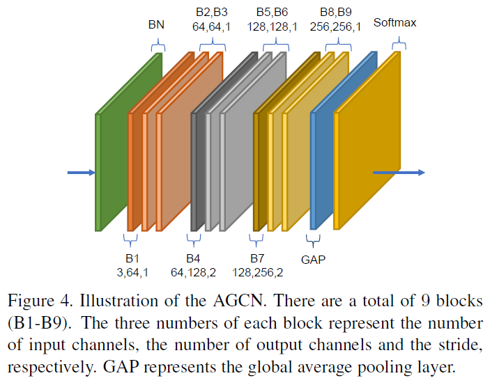
temporal dimension에 대한 convolution은 ST-GCN에서와 같죠. 가령, K_t x 1 convolution이 C x T x N feature maps에 대해 performing되죠. spatial GCN 과 temporl GCN 모두 BN layer와 Relu layer가 뒤따릅니다. Fig 3. 에서 볼 수 있듯이, 하나의 basic block은 하나의 spatial GCN ( Convs ), 하나의 temporal GCN ( Convt ) 그리고 drop rate이 0.5로 set 된 dropout layer 의 combination입니다. training을 stabilize하기 위해, residual connection이 각 block에 추가되죠.

Adaptive graph convolutional network
AGCN은 이들 basic blocks의 stack이죠. 이는 Fig 4에서 볼 수 있죠. 총 9 개의 blocks를 가지고 있죠. output channels의 수는 64, 64, 64, 128, 128, 128, 256, 256, 256 입니다. data BN layer는 input data를 normalize하기 위해 처음에 추가되죠. global average pooling layer는 동일 size로 different samles의 fueature maps를 pool 하기 위해 마지막에 performed 됩니다. final output은 prediction을 obtain하는 softmax classifier로 sent 됩니다.
Two-stream networks
bone information과 같은 second-order information은 skeleton based action recognition에서 중요하지만 이전 연구에서 무시되어 왔죠. 이 논문에서, 저자들은 second-order information을 modeling을 제안하죠. 이는 two-stream framework을 통해 modeling되고 recognition을 enhance하죠.
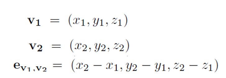
구체적으로, 각 bone이 two joints와 bound 되어 있기 때문에, 저자들은 skeleton의 center of gravity와 가까운 joint는 source joint로 center of gravity와 먼 joint를 target joint로 define합니다. 각 bone은 vector로 represented 되는데 source joint로 부터 target joint를 pointing 하죠. 이는 length information을 contain할 뿐만아니라, direction information 역시 contain하죠. 예를 들면, source joint v1 , target joint v2가 주어지면, bone의 vector는 e_v1,v2로 계산되는 데 아래와 같습니다.
skelton data의 graph가 cycles을 가지기 않기 때문에, 각 bone은 unique target joint로 assigned 될 수 있죠. joints의 number는 bones의 number보다 하나가 더 많죠. 왜냐하면 central joint는 어떤 bones과도 assigned 되지 않기 때문이죠. network의 design을 simplify하기 위해, 저자들은 cnetral joint에 0의 value로 empty bone 추가합니다. 이런 방식으로, bones의 graph와 network는 joints의 graph와 network와 같이 desinged 됩니다. 저자들은 J-stream과 B-stream을 사용하는데 이는 joints와 bones의 network를 represent 합니다. overall architecture는 Fig 5.에서 볼 수 있죠.
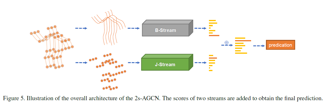
sample이 주어지면, 저자들은 먼저 joints의 data에 기반해 bones의 data를 먼저 계산합니다. 그리고 난 뒤, joint data와 bone data가 J-stream 과 B-stream의 input으로 던져지죠. 마지막으로, two streams의 softmax scores는 fused socre를 obtain하기 위해 그리고 action label을 prediction 하기 위해 추가되죠.
나머지 부분은 생략할게요.
다른 논문들도 참고하셔요
MST-GCN에 이해가 안가는 코드가 있었는데
여기의 code를 base로 해서 그런거였네요.
하 이걸 활용할 수 가 있어야되는데
서버에서 좀하지 꼭..하


