이번 논문은 st-gcn이죠
action recognition을 하는데
왜 갑자기 traffic forcast냐
이 archietecture가 중요하기 때문이죠
Abstract
적시에 정확한 traffic forecast는 중요하죠. high nonlinearity 와 traffic flow의 complexity, traditional methods는 mid-and-long term prediction task 의 requirements를 만족시키지 못하죠. 종종 spatial and temporal dependencies를 무시하기도 하고요. 이 논문에서, 저자들은 Spatio-Temporal graph Convolutional Networks (STGCN)을 제안합니다. traffic domain에서 time series prediciton problem을 다루죠. regular convolutional 과 recurrent units를 applying 하는 대신에, 저자들은 graphs에 대해 problem을 formulate하고 complete convolutional structures를 가진 model 을 construct합니다. 이는 fewer parameters를 가지고 훨씬 빠른 training이 enable하게 하죠. 실험은 STGCN이 comprehensive spatio-temporal correlations를 multi-scale traffic networks의 modeling을 통해 effectively 하게 captures하고 SOTA baselines을 뛰어넘었다고 합니다.
Introduction
Transportation은 everbody's daily life에 필수적인 역할을 하죠. 2015 에 survey에 따르면, U.S. drivers는 평균적으로 약 48분을 운전대를 잡고 시간을 보낸다고 하죠. 이런 상황에서, traffic conditions의 accurate real-time foercast는 도로 이용자, 개인 비서 그리고 정부에게 있어 가장 중요하죠. 광범위하게 사용되는 transportation services, 가령 flow control, route planning, navigation과 같은 것들이 있는데, 이들은 high-quality traffic condition evaluation에 굉장히 의존적이죠. 일반적으로, multi-scale traffic forecast는 urban traffic control과 guidance의 premise이자 foundation이죠. 또한 Intelligent Transportation System의 하나의 중요한 기능이기도 하고요.
traffic study에서, traffic flow의 fundamental variables, speed, volume, 그리고 density는 typically incators로써 선택되죠. 이는 traffic conditions를 monitor하고 future를 predict하고요. prediction의 length에 기반해, traffic forecast는 two scaleds로 분류되죠. short-term( 5 ~ 30 min ), medium and long term ( over 30 min ) . 일반적인 statistical approaches는 short interval forecast에서 좋은 성능을 보입니다. 그러나, traffic flow의 complexity와 uncertatinty때문에, 이런 methods는 상대적으로 long-term predictions에 대해 less effective하죠.
Previous studies 중 mid-and-long term traffic prediction에 관한 것은 대략 tow categories로 나눠집니다: dynamical modeling과 data-driven methods. Dynamical modeling은 mathmatical tools를 사용하죠 ( differential equations 같은 ) 그리고 computational simulation으로 traffic problems를 formulate 한 physical knowledge 역시 사용합니다. steady state을 achieve하기 위해, simulation process는 sophisticated systematci programming을 요구할 뿐만아니라, massive computational power를 역시 소모되죠. Impractical assumptions와 simpifications 는 prediction accuracy를 degrade하죠. 그럼으로 traffic data collection의 발전과 techniques storage의 발전을 토대로, 많은 연구자들이 그들의 attention을 data-driven approaches로 전향했죠.
Classic statistical and machine learning models는 data-driven methods의 두 대표주자인데요. timeseries analysis에서, autoregressive integrated moving average ( ARIMA ) 와 its variants는 classical statistics에 기반한 가장 consolidated approaches죠. 그러나 이런 종류의 model은 spatio-temporal correlation을 고려하는 데 실패했죠. 그럼으로, 이 approaches는 highly nonlinear traffic flow의 representabilty에 제약이 있어왔고요. 최근, classic statistical models는 traffic prediction task에 대해 machine learning methods에 의해 도전을 받아왔죠. 더 높은 prediction accuracy와 더 복잡한 data modeling은 이 models( KNN, SVM, NN )에 의해 성취되었죠.
Deep learning approaches
Deep learning approaches는 various taffic task에서 광범위하게 성공적으로 applied 되었죠. 그러나, input으로 부터 동시에 spatial and temporal features를 extract하는 dense networks에 어려움이 있죠. 게다가, narrow constraints 나 심지어 spatial attributes의 complete absence 안에서, 이런 networks의 represntative abiility는 심각하게 다뤄졌고요
spatial features의 장점을 취하기 위해, 몇몇 연구가는 CNN을 traffic netowrk에서 adjacent relations을 capture하는 데 사용했죠. time axis에 대해 RNN을 사용했고요. LSTM과 1-D CNN을 결합함으로써, Wu 와 Tan은 shorterm traffic forecast를 위한 CLTFP 를 제안했죠. 비록 직관적으로 적용되긴 했지만, CLTFP는 여전히 spatial and temporal regularities에 대해 시도하고 있죠. 후에, Shi는 convolutional LSTM을 제안했고 FC-LSTM의 확장판이죠. 그러나, normal convolutional operation은 model이 grid structures만을 처리하도록 제약했고요. 그러는 동안 sequence learning을 위한 RNN은 iterative training을 요구했죠. 이는 steps에 의한 error accumulation을 도입되었죠. 추가적으로, RNN-based networks는 train하기 어렵고 computationally heavy하죠.
이 문제를 해결하기 위해, 저자들은 temporal dynamics와 traffic flow의 spatial dependencies를 effectively model하는 몇몇 전략을 소개한다고 하네요. spatial information을 완전하게 사용하기 위해, 저자들은 각각 다루기 보다 general graph로 traffic fnetwork를 model 한답니다. RNN의 inherent deficiencies를 다루기 위해, 저자들은 time axis에 convolutional structure를 사용한다고 하고요. 이 모두를 통틀어, 저자들은 STGCN을 제안한다고 합니다. 이 architecture는 spatio-temporal convolutional blocks로 이뤄져있고 graph convolutional layers과 convolutional sequence learning layer의 combination이라고 합니다. 자신들이 아는 한, traffic study에서 graph-structured time series로부터 spatio-temporal features를 추출하는 purely convolutional structures를 처음으로 적용했다고 하네요.
Preliminary
Traffic Prediction on Road Graphs
Traffic forecast는 typical time-series prediction problem이죠. 가령 previous M traffic observation이 아래와 같이 주어지면 the most likely traffic measurements ( speed or traffic flow ) 를 next H time steps에 predicting하는 것등이 있죠.
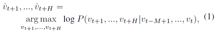
v_t ( R^n )은 time step t에서 n road segments의 observation vector입니다. single road segment에 대한 historical observation 의 각 요소죠.
이 연구에서, 저자들은 graph에 대해 traffic network를 정의합니다. 그리고 structured traffic time series에 초점을 맞추죠. observation v_t는 독립적이진 않고 graph에서 pairwise connection에 의해 linked 되죠. 그럼으로 data point v_t는 graph signal로써 여겨지죠. 이는 weights w_ij를 가지는 G ( undirected graph or directed one )에 대해 정의되죠. 이는 그림 1에서 볼 수 있고요.

t-th time step에서, graph G = ( V_t, epsilon, W ), V_t는 vertices의 finite set이고 traffic network에서 n monitor stations으로부터 observations에 해당하죠. epsilon은 edge의 set으로, stations 간의 connectedness를 나타내고요. W ( R ^ n x n )은 G_t의 weighted adjacency matrix을 표기합니다.
Convolutions on Graphs
regular grids를 위한 standard convolution은 general graphs에 적용될 수 없죠. structed data forms에 CNNs를 일반화 하는 방법을 사용하는 basic한 두 가지 approaches가 있죠. 하나는 convolution의 spatial definition을 expand하는 것이고 다른 하나는 graph Fourier transforms를 가진 spectral domain에서 manipulate하는 것이죠. 전자의 approach는 vertices를 certain grid forms로 rearranges합니다. certain grid forms는 normal convolutional operations 에 의해 processed 될 수 있죠. 후자는 spectral domains에 convolution을 apply한 spectral framework를 도입합니다. 이는 종종 spectral graph convolution으로 불리기도 하죠. 몇몇 뒤따른 연구는 graph convolution을 더 유망하게 만드는데 O(n^2)로부터 linear하게 computational complexity를 줄였죠.
저자들은 graph convolution operator의 notion을 도입합니다. 이는 spectral graph convolution의 conception에 기반하죠. kernel theta를 가진 signal x ( R^n )의 multiplication이고 식으로는 아래와 같습니다.

graph Fourier basis U ( R ^ n x n )는 normalized graph Laplacian L 의 eigenvectors죠 식으로는 아래와 같습니다.

I_n은 identity matix이고 D는 L의 eigenvalues 에 대한 diagonal matrix 이고 filter theta( ) 는 diagonal matrix이죠. 이런 정의를 통해, graph signal x 는 theta와 graph Fourier transform U^Tx 간의 multiplication을 하는 kernel theta에 의해 filtered 되죠.
Proposed Model
Network Architecture
이 section에서, 저자들은 STGCN에 대해 상세히 설명하는데요. Fig 2에서 볼 수 있듯이, STGCN은 몇 개의 spatio-temporal convolutional blocks로 구성되어 있죠. 각각은 두 개의 gated sequential convolution layers와 하나의 spatial graph convolution layer를 그들 사이에 가진 'sandwich' structure로 구성되고요. 각 module에 대한 상세 설명은 아래서 한다네요

Graph CNNs for Extracting Spatial Features
traffic network는 일반적으로 graph structure로 조직화되죠. graphs 로 road networks를 formulate하는 것은 수학적으로 자연스럽고 타당하죠. 그러나, 이전 연구들은 traffic networks의 spatial attribute을 무시합니다: connectivity와 globality 를 간과하는 데, multiple segment나 grids로 나눴기 때문이죠. grids에 대해 2-D convolutions를 활용할때 조차, data modeling의 compromises 때문에 spatial locality만 대략적으로 capture할 뿐이죠. 이에 따라, STGCN에서는, graph convolution이 highly meaningful patterns와 features를 space domain에서 extract하는 graph structured data에 대해 직접적으로 사용됩니다. 비록 Eq.2에 의한 graph convolution에서 kernel theta의 computation이 graph Fourier basis를 가진 multiplications O(n^2) 때문에 expensive할 수 있지만, 두 가지 approximation strategies가 이 issue를 극복하기 위해 적용되죠.
Chebyshev Polynomials Approximation
filter를 localize하고 parameters의 수를 줄이기 위해, kernel theta는 lambda( A처럼 생긴 넘 ) 의 polynomial 에 restricted 될 수 있죠. 식으로 표현하면 아래와 같아요

theta는( R^K) polynomial coefficients의 vector입니다. K는 graph convolution의 kernel size이고요. 이는 central nodes로부터 convolution의 maximum radius를 결정하죠. 전통적으로 chebyshev polynomial T_k( x )는 kernels를 truncated expansion of order K-1로써 approximate하는데 사용하는데 식은 아래와 같죠

lambda_max는 L의 largest eigenvalue를 표기하죠. graph convolution은 아래와 같이 쓰여질 수 있습니다.

여기서 T_k(~L) ( R^nxn) 은 scaled Laplacian에서 evaluated된 order k 의 Chebyshev polynomial 입니다. polynomial approximation을 통한 K-localized convolutions 를 recursively 하게 computing 함으로써, Eq 2의 cost는 Eq 3처럼 줄 수 있죠.
1^st-order Approcimation
layer-wise linear formulation은 graph Laplacian의 first-order approximation을 가진 mutiple localized graph convolutional layers를 stacking함으로써 정의될 수 있죠. 구체적으로, deeper architecture는 polynomials에 의해 주어진 explicit parameterizaion에 제한되는 것 없이 depth 에서 spatial information을 recover하기 위해 constructed 될 수 있죠. neural networks에서 scaling과 normalization 때문에, 저자들은 lambda_max ~= 2로 가정할 수이 었죠. 따라서 Eq 3은 아래와 같이 단순화 될 수 있습니다.

theta0, theta1 은 kernel의 두 개의 shared parameters입니다. parameters를 constrain 하고 numerical performances를 stabilize하기 위해, theta0, theta1은 theta = theta0 = - theta1로 정함으로써 single parameter theta로 대체될 수 있죠; W와 D는 renomalized 되죠. 식은 각각 아래와 같고요

그런다음, graph convolution은 아래처럼 대체해서 표현할 수 있게 되죠.

K-localized convolutions로써 유사한 효과를 내는 first-order approximation을 vertically로 활용한 graph convolutions의 stack을 applying하는 것을 center nodes의 ( K-1 ) -order neighborhoods로부터 imformation을 사용하는 all에 horizontally 적용하죠. 이 scenario에서, K 는 successive filtering operations나 model에서 convolutional layers의 수입니다. 더불어, layer-wise linear structure는 parameter-economic 하고 large-scale graphs에 대해 highly efficient합니다. approximation의 order가 one으로 제한되기 때문이죠.
Generalization of Graph Convolutions
graph convolution operator "*g" 는 x( R^n)에서 정의 되는데, x는 multi-dimensional tensors로 extended됩니다. C_i channels를 가진 signal X ( R^n x C_i ) 에 대해, graph convolution은 아래와 같이 일반화 될 수 있죠.

Chebyshev coefficients theta_i,j( R^K ) 의 C_i x C_o vectors( C_i, C_o 는 feature map에 대한 input과 output 의 size )입니다. 2-D variables를 위한 graph convolution은 " theta * g X "( R^ K x C_i x C_o )로 표기됩니다. 구체적으로, traffic prediction의 input은 road graphs의 M frame으로 구성되어 있는데요. 각 frame v_t는 matrix로 여겨지는 데. column i 는 i^th node에 대한 v_t의 C_i-dimensional value 로 여겨지죠. X ( R^nxC_i ). 각 M의 time step에 대해, equal graph convolution operation 은 same kernel theta를 가지며 X_t( R^nxC_i)에 병렬적으로 imposed됩니다. 따라서 graph convolution은 3-D variables에서 일반화됩니다. Theta * g Chi 로 표기되고 Chi (R^MxnxC_i) 입니다.
Gated CNNs for Extracting Temporal Features
RNN-based models가 time-series analysis에서 일반적이긴하지만, recurrent network 는 time-consuming iterations, complex gate mechanism, 그리고 dynamic changes에 slow response 와 같은 문제가 있죠. 반면, CNNs는 fast training, simple structures, 그리고 이전 steps에 no dependency constraint에 우위가 있죠. 저자들은 entire convolutional structures를 times axis에 대해 사용하는데, traffic flow의 temporal dynamic behaviors를 capture하죠. 이 specific design은 hierarchical representations로 formed 된 multi-layer-convolutional structures를 통해 parallel 하고 controllable training procedures를 가능하게 하죠.
temporal convolutional layer는 non-linerarity로써 GLU이 뒤따르는 width-K_t kernel을 가진 1-D causal convolution을 포함하죠. graph g에서 각 node에 대해, temporal convolution이 input elements의 K_t neighbors 사용합니다. 이 때 padding이 사용되지 않기 때문에 K_t-1 time으로 sequences의 lenth가 줄어들죠. 따라서, each node에 대해 temporal convolution의 input은 C_i channels를 가진 lengh-M sequence로써 여겨지죠. ( Y (R^MxC_i) ). convolution kernel gamma ( R^K_t x C_i x 2C_o )은 input Y를 single output element [ P Q ] ( R ^ (M - K_t + 1 )x(2C_o) )로 map 하기위해 designed되죠. ( P, Q는 channels를 반으로 나눈 같은 size를 가진 split 이죠 ). 결과적으로 temporal gated convolution은 아래와 같이 정의됩니다.

P, Q 는 GLU에서 gate의 inpute 이죠; double dot은 element-wise Hadamard product입니다. sigmoid gate는 , sigma( Q ) , current states 의 어떤 input P가 time series에서 compositional structure 과 dynamic variances를 discovering 하는 거과 관련 있는 지를 control합니다. non-linearity gates는 stacked temporal layers를 통해 filed된 full input의 exploiting에 contribute하죠. 나아가, residual connections는 stacked temporal convolutional layers 중에 implemented 됩니다. 유사하게, temporal convolution은 3-D variables로 generalized되죠.
Spatio-temporal Convolutional Block
spatial and temporal domains 모두로 부터 features를 fuse하기 위해, spatio-temporal convolutional block (ST-Conv block) 은 graph-structured time series를 동시에 process하기 위해 constructed됩니다. block은 그 자체로 stacked 될 수 있거나 extended 될 수 있죠. particular cases의 scale과 complexity에 기반해서 말이죠.
spatial layer는 tow temporal layers를 bridge 합니다. 이는 temporal convolutions를 통해 graph convolution으로 부터 fast spatial-state propagation이 가능하게 해주죠. "sandwich" structure는 network가 graph convolutional layer를 통해 channels C의 downscaling과 upscaling을 함으로써 scale compression과 feature squeezing을 가능하게 하는 bottleneck strategy를 apply 할 수 있도록 돕죠. 게다가, layer normalization은 ST-Conv block에서 overfitting을 prevent하기 위해 사용됩니다.
ST-Conv blocks의 input과 output은 all 3-D tensors인데요. input v^l 은 block l의 input이고, output v^l+1 은 R^(M-2(K_t-1)) x n x C^l+1 에 속하며 아래와 같이 계산되죠.

gamma^l_0, gamma^l_1 은 block l 에서의 upper 과 lower temporal kernel이고 theta^l은 graph convolution의 spectral kernel입니다. ReLU( )는 rectified linear units function을 표기합니다. two ST-Conv blocks를 쌓은 뒤에, FC layer를 가진 extra temporal convolution layer 붙입니다. 이 temporal convolution layer는 last ST-Conv block의 output을 single-step prediction으로 map하죠. 그런 뒤, 저자들은 final output Z를 얻습니다. ( R^nxc ) 그리고 c-channels를 따라 linear transformation을 applying함으로써 n nodes에 대해 speed prediction을 calcurate하죠. 저자들은 L2 loss를 사용하는데 이는, model의 performacne를 측정해주죠. 따라서 loss function은 아래와 같이 쓸수 있습니다.

여기까지 할게요.
좀 오래된 모델이긴 하지만
skeleton based model들에서 많이 사용하기에
리뷰해봤습니다


