Centernet 공식 github에 있는 논문이죠
앞에서 다룬 CenterNet 논문도 관련 논문이지만
이 논문은 공식 github에 있는 논문이기 때문에
한번 보도록하죠
Abstract
Detection은 objects를 axis-aligned boxes로써 identifies하죠. Most successful object detectors는 potential object locations의 exhaustive list를 enumerate하고 각각을 classify 하죠. 이런 방식은 wasteful하고 inefficient, 하며 additional post-processing을 requires 합니다. 이 논문에서는, 다른 approach를 채택하는데요. object를 single point로써 model합니다. single point는 bounding box의 center point를 가리키죠. 저자들의 detector는 center points를 find하는 keypoint estimation을 사용하고 size,3D location, orentation, 심지어 pose와 같은 all other object properties로 regress합니다. center point based approach는 CenterNet이라 불리고 end-to-end differentiable하고, corresponding bounding box based detectors보다 simper, faster 그리고 more accurate 하죠.
Introduction
Object detection은 많은 vision tasks에서 강력합니다. 가령 instance segmentation, pose estimation, tracking 그리고 action recognition과 같은 task들이 있겠죠. Current object detectors는 각 object를 axies-aligned bounding box를 통해 represent하죠. bounding boxes들은 object를 감싸고 있고요. detectors는 object detection을 potential object bounding boxes의 extensvie number에 대한 image classification으로 단순화하죠. 각 bounding box에 대해, classifier는 image content가 specific object인지 background인지를 determine하죠. one stage detectors는 anchor라 불리는 possible bounding boxes의 complex arrangement를 image에 slide하죠. 그리고 그들을 직접 classify 합니다. 물론 box content를 specifying 하지 않죠. Two-stage detectors는 각 potential box에 대해 image features를 recompute합니다. 그런다음 이 features를 classify 하죠. NMS라 불리는 post-processing 이 bounding box IoU 를 computing함으로써 same instance에 대해 duplicated detections를 remove하죠. 이 post-processing은 differentiate과 train하기 어렵기에, 많은 current detectors는 end-to-end로 trainable 하지 않죠. 그럼에도 불구하고, 5년간, 이 idea는 good empirical sucess를 달성했죠. object detectors에 기반한 Sliding window는 다소 wasteful한데, sliding window는 all possible object locations와 dimensions를 enumerate 할 필요가 있기 때문이죠.
이 논문에서, 저자들은 더 간단하고 더 efficient한 alternative를 제공합니다. objects를 single point로 represent하는데 FIgure 2에서 볼 수 있죠.
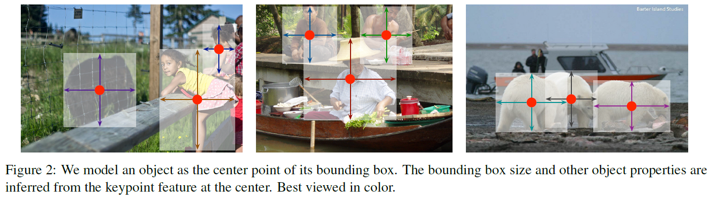
object size, dimension, 3D extent, orientation, 그리고 pose와 같은 Other properties는 center location에 image features로부터 직접 regressed 됩니다. 그러면, Object detection은 standard keypoint estimation problem이 되죠. image를 input으로 fully convvolutional network에 넣어줍니다. network는 heatmap을 생성하죠. 이 heatmap에서 Peaks는 object centers와 상관이 있죠. 각 peak에서 Image features는 objects bounding box height와 weight를 예측하죠. model은 standard dense supervised learning을 활용해서 trains합니다. Inference는 single network forwad-pass 이며, non-maximal suppresion 과정이 없죠.
저자들의 method는 general 하고 other task로 약간의 노력만 있으면 extended 될 수 있죠. 저자들은 3D object detection, multi-person human pose estimation 에 대한 experments를 제공합니다. 이는 각 center point에서 additional outputs를 predicting 함으로써 가능하게 되죠. Fig 4에서 볼수 있죠

3D bounding box estimation을 위해, object absolute depth, 3D bounding box dimensions 그리고 object orientation로 regress 하죠. pose estimation을 위해, 2D joint locations을 center로 부터 offset으로써 고려합니다. 그리고 center point location에서 2D joint locations로 regress하죠.
CenterNet의 simplicity는 빠른 속도를 자랑합니다. Figure 1에서 볼 수 있죠. 성능에 대한 내용은 생략합니다.

Related work
Object detection by region classification
RCNN 은 region candidates의 large set으로부터 object location을 enumerate 하고 crops them 이후에 각각을 deep network를 활용하여 classifies합니다. Fast-RCNN은 image features를 crops 하죠. 그러나 두 방법 모두 sollow-level region proposal mehods에 의존하죠.
Object detection with implicit anchors
Faster RCNN은 reion proposal을 detection network에서 generate하죠. 이는 low-resolution image grid에서 fixed-shape bounding boxes를 samples 하고 각각을 foreground인지 아닌지를 classifies합니다. anchor는 any ground truth object와 ovelap 을 기준으로 a>0.7 이면 foreground로 a<0.3이면 background 로 labeled 됩니다. 때로는 무시하기도 하고요. Each generated region proposal은 다시 classified 됩니다. proposal classifier를 multi-class classification 으로 changing하는 것은 one-stage detectors의 basis를 forms하죠. Several imrovements 는 anchor shape priors, different feature resolution 그리고 different samples 중에 loss re-weighting 을 포함하죠
CenterNet은 anchor-based one-stage approaches와 매우 연관되어 있습니다. center point는 single shape-agnostic anchor로 볼 수 있죠, 이는 Figure 3에서 볼 수 있습니다.

그러나 중요한 차이가 있습니다. 먼저 CenterNet은 오로지 location에만 기반하여 ancohr를 assigns 합니다. box의 overlap은 고려 대상이 아니죠. foreground나 background classification에 대한 manual 한 thesholds가 존재하지 않습니다. 두 번째, object당 오직 하나의 positive anchor를 가집니다. 따라서 NMS가 필요하지 않죠. keypoint heatmap에서 local peaks만을 단순하게 extract합니다. 세 번째, CenterNet은 larger output reolution을 사용하는 데, 이는 multiple anchors에 대한 필요성을 제거하죠.
Object detection by keypoint estimation
CenterNet은 object detection을 위해 key point estimation을 처음 시도한 framework이 아닙니다. CornerNet은 두 개의 bounding box corner를 keypoints로써 detect합니다. 반면에 ExtremeNet은 top-, left-, bottom-, right-most와 center point를 모든 objects에 대해 detects하죠. 이 방법들 모두 CenterNet과 같은 robust keypoint estimation을 기반으로 하죠. 그러나, 그들은 keypoint detection 이후에 combinatiorial grouping stage를 요구하죠. 각 algorithm을 상당히 느리게 하고요. CenterNet은 반면, object당 singel center point를 grouping 이나 post-processing 없이 extracts하죠
Monocular 3D object detection
3D bounding box estimation은 autonomous driving,에 강력합니다. Deep3Dbox는 slow-RCNN style framework를 사용하는데, 이는 처음에 2D objects를 detecting하고 각 object를 3D estimation network에 입력으로 던져주죠. 3D RCNN은 additional head를 3D projection에 의해 뒤따라 나오는 Faster-RCNN에 추가합니다. Deep Manta는 많은 task에 대해 trained된 coarse-to-fine Faster-RCNN을 사용합니다. CenterNet은 Deep3Dbox나 3DRCNN의 one-stage version과 유사합니다. 이와 같이, CenterNet은 경쟁 모델에 비해 훨씬 단순하고 빠르죠.
Preliminary
I ( W x H x 3 )이 넓이 W와 높이 H를 가진 image라고 해봅시다. 목표는 keypoint heatmap hat Y ( [0,1]^W/R x H/R x C )를 produce하는 것이죠. 여기서 R은 output stride이고 C는 keypoint types의 number입니다. Keypoint types는 pose estimation에서 C=17 human joints를 포함합니다. 혹은 object detection에서 C = 80 과 같은 object categories를 포함하기도 하죠. 저자들은 R=4 를 default output stride 로 사용하죠. output stride는 output prediction을 factor R로 downsample 하죠. prediction hat Y_x, y, c = 1은 detected keypoint에 해당하며, hat Y_x,y,c = 0은 background에 해당하죠. 저자들은 several different fully-convolutional encoder-decoder network를 사용하는데 이는 hat Y를 image I로 부터 predict하죠. : stacked hourglass network, up-convolutional residual networks 그리고 deep layer agrregation ( DLA ) 등을 사용하죠.
저자들은 keypoint prediction network 를 train합니다. 각 class c의 ground truth keypoint p ( R^2 )에 대해, 저자들은 low-resolution equivalent ~p = [ p/R ] 을 계산하죠. 그런다음 all ground truth keypoint를 heatmap Y ( [ 0, 1 ]^ W/R x H/R x C에 Gaussian kernel Y_xyc = exp ( - ( (x-~p_x)^2 + (y-~p_y)^2 / 2simga^2_p) )를 사용해서 splat합니다. 여기서 sigma_p 는 object size-adaptive standard deviation이죠. 만일, same class를 가진 두 개의 gaussians 이 overlap하면, element-wise maximum을 취합니다. training objective는 focal loss를 가진 penalty-reduced pixel-wise logistic regression이고 식은 아래와 같습니다.
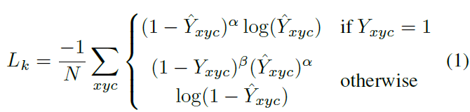
여기서 alph와 beta는 focal loss의 hyper-parameter입니다. N은 image I에서 keypoints의 개수이고요. N으로 normalization은 all positive focal loss isntances를 1로 normalize하기 위해 선택됩니다. alpha는 2, beta는 4로 set 했죠.
output sitride에 의해 야기되는 discretization error를 recover하기 위해, 각 center point에 대해 local offest hat O ( R^W/R x H/R x 2 )를 추가적으로 prdict하는데요. All classes c는 same offset prediction을 공유합니다. offset은 L1 loss를 활용해 trained 되고 식은 아래와 같죠
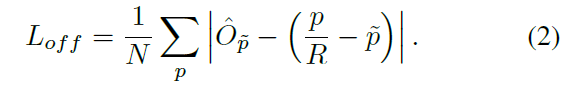
supervision은 keypoints locations ~ p에서만 동작합니다. 다른 모든 location은 무시되죠.
다음 section에서 keypoint estimator를 general purpose object detector로 extend하는 방법을 보여준다고 하네요
Objects as Points
( x^(k)_1, y^(k)_1, x^(k)_2, y^(k)_2 ) 를 category c_k를 가진 object k의 bounding box 라고 해봅시다. its center point는 p_k에 놓여 있고 p_k = ( (x^(k)_1 + x^(k)_2 )/2 , (y^(k)_1 + y^(k)_2)/2 ) 겠죠. all center points를 predict하는 key point estimator hat Y를 사용하죠. 그 다음, object size s_k로 regress 하는 데, 각 object k에 대해 s_k = ( x^(k)_2 - x^(k)_1, y^(k)_2 - y^(k)_1 ) 이죠. computation burden을 limit하기 위해, 저자들은 singel size prediction hat S ( R^ W/R x H/R x 2 ) 를 모든 object categories에 대해 사용합니다. center point에서 L1 loss를 사용하는데 Objective 2와 유사하죠.
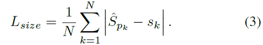
저자들은 scale을 normalize하지 않고 raw pixel coordinates를 직접 사용합니다. 대신에 loss를 constant lambda_size로 scale하죠. 전체 training objective는 아래와 같습니다.

lambda_size = 0.1, lambda_off = 1로 set 하죠. keypoints hat Y, offset hat O 그리고 size hat S를 predice하는 single network를 사용합니다. network는 C+4 outputs를 각 location에서 predicts합니다. All outputs는 common fully-convolutional backbone network를 공유하죠. 각 modality에 대해, backbone의 features는 separate 3 x 3 convolution, Relu 그리고 또 다른 1 x 1 convolution을 통과하죠. Figure 4는 network output의 overview를 보여줍니다.
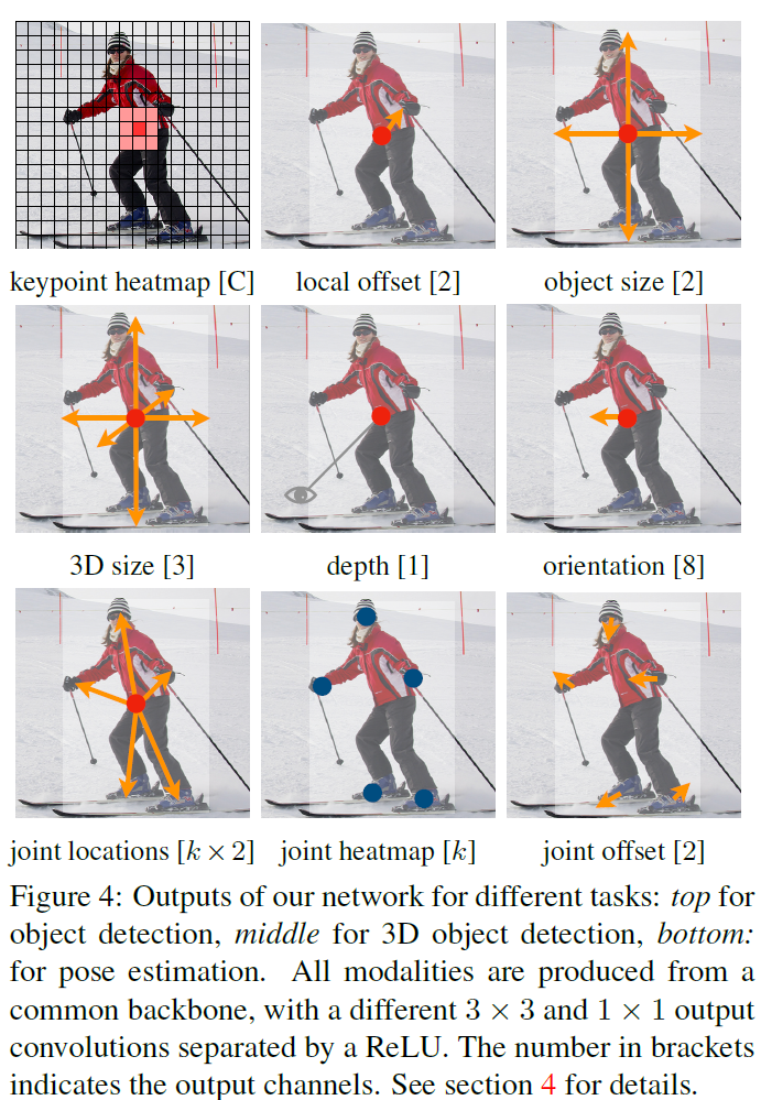
Section 5와 supplementary material은 additional architectural details를 포함하죠.
From points to bounding boxes
inference time에, 저자들은 먼저 heatmap에서 각 category에 대해 독립적으로 peaks를 extract합니다.저자들은 all responses 를 detect하는데 all responses의 value는 its 8-connectece neibors 보다 크거나 같죠. 그리고 top 100 peaks를 keep합니다. hat P_c를 class c의 center points hat P = { (hat x_i, hat y_i) }^n_i=1 로 detected된 n 개의 set 이라고 해봅시다. 각 keypoint location은 integer coordinates ( x_i, y_i )로 주어지죠. 저자들은 key point values hat Y_x_iy_ic 를 its detection confidence의 measure로써 사용합니다. 그리고 location에 bounding box 를 생성하고 식은 아래와 같죠.
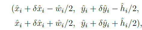
여기서 ( delta hat x_i, delta hat y_i ) = hat O _hat x_i, hat y_i 는 offset prediction 이고 ( hat w_i, hat h_i ) = hat S_ hat x_i, hat y_i 는 size prediction이죠. all outputs는 keypoin estimation으로부터 직접 produced 되는데 IoU-based NMS나 다른 post-processing이 필요하지 않죠. peak keypoint extraction은 sufficient NMS alternative로서의 역할을 하죠. 그리고 3 x 3 max pooling operation을 사용하여 device에서 efficiently 하게 implemented 될 수 있죠.
3D detection
3D detection 은 objects 당 three-dimensional bounding box 를 추정하죠. 또한 center point당 additional attributes를 요구합니다. 가령 depth, 3D dimension, and orientation 등이 있죠. 저자들은 separate head를 추가하는 데요. depth d 는 center point 당 singel scalar입니다. 그러나, depth는 직접 regress 하기 어렵죠. 대신에 output transformation을 사용합니다. 저자들은 depth를 keypoint estimator의 additional output channel hat D ( [ 0,1 ] ^ W/R x H/R 로 계산합니다. Relu 로 separated 된 두 개의 convolutional layers를 다시 사용하죠. 이전 modalities와 다르게, inverse sigmoidal transformation을 output layer에 사용합니다. depth estimator를 train 하는데 sigmoidal transformation 후에 original depth domain에 L1 loss를 사용하죠.
object의 3D dimensions는 three scalars인데요. 저자들은 직접적으로 absolute values로 regress 합니다. separated head hat gamma ( R^ W/R x H/R x 3 ) 과 L1 loss 를 사용하죠.
orientation은 single scalar 입니다. 그러나, regress 하기 어렵죠. Mousavian 연구를 참조합니다 그리고 orentation을 in-bin regression을 가진 two bin으로 represent하죠. 특별히, orientation은 8 scalars를 사용해 encoded됩니다. 각 bin에 대해 4 개의 scalars를 가지죠. 하나의 bin에 대해, 두개의 scalars는 softmax classification을 사용하고 나머지 두 개의 scalar는 각 bin안에서 angle로 regress 됩니다.
Human pose estimation
Human pose estimation은 image안에서 모든 human instance에 대해 k개의 2D human joint locations을 estimate하는 것을 목표로합니다. 저자들은 pose를 center point의 k x 2-dimensional property로 consider하고 각 keypoint를 offeset을 가지고 center point로 parametrize합니다. joint offsets로 직접 regress 하는 데 hat J ( R ^ W/R x H/R x k x 2 )는 L1 loss를 활용하죠. loss를 masking함으로써 invisible keypoint는 ignore합니다. 이는 regression-based one-stage multi person human pose estimator 의 결과가 됩니다.
keypoints를 refine 하기 위해, 저자들은 k 개의 human joint heatmaps hat pi ( R ^ W/R x H/R x k )를 estimate합니다. standard bottom-up multi-human pose estimation을 사용하죠. human joint heatmap을 focal loss와 Section 3에서 설명한 center detection과 유사한 local pixel offset 을 가지고 train합니다.
저자들은 그리고 나서 initial predictions를 이 heatmap에서 closest detected keypoint 로 snap 합니다. 여기서 center offset은 grouping cue로 동작하죠. 이는 individual keypoint detections를 closest person instance로 assign합니다. 구체적으로, ( hat x, hat y )를 detected center point라고 합니다. 먼저 all joint location l_j = ( hat x, hat y ) + hat J_hat x hat y j ( j = 1 , ... , k ) 로 regress 합니다. 또한 all keypoint locations L_j = { ~l_ ji } ^ n_j _i = 1 ( confidence > 0.1 ) 을 각 joint type j 에 대해 해당 heatmap hat pi 로부터 extract하죠. 그런 다음, regressed location l_j 를 closest detected keypoint ( arg min ( l - l_j )^2 )로 각각 assign 하는데 detected keypoint는 detected object의 bounding box 안에서 joint detections를 considering 하죠.
Implementation details
4 개의 architecture로 실험했다고 합니다. 저자들은 ResNets과 deformable convolution layers를 사용한 DLA-34 모두를 modify 했고 Howrglass network을 있는 그대로 사용했다고 하네요.
Hourglass
stacked Hourglass Network는 input을 4 x로 downsamples 하죠. 이는 두 개의 sequential hourglass module를 통해 이뤄지고요. 각 hourglass module은 skip connections를 가진 symmetric 5 - layer down- and up- convolutional network 이죠. 이 network는 꽤 크지만, best keypoint estiamtion performance를 보여주죠
ResNet
Xiao et al 연구는 higher-resolution output ( output stride 4 ) 를 허용하는 three up-convolutional networks 가진 standard residual networs를 augment 했는데요. 저자들은 먼저 three upsampling layers의 channels를 256, 128, 64 로 바꿨죠. 이는 computation을 절약하기 위함이었고요. 그 다음 3 x 3 deformable convolutional layer를 256, 128, 64 channel을 가진 up-convolution 전에 추가 했죠. up-convolutional kernels는 bilinear interpolation으로 initialized 됩니다.
DLA
Deep Layer Aggregation ( DLA )는 hierarchical skip connections를 가진 image classification network 인데요. 저자들은 DLA의 fully convolutional upsampling version을 dense prediction을 위해 사용합니다. 이는, feature map resolution을 symmetrically하게 increase하는 iterative deep aggregation을 사용합니다. 저자들은 lower layers부터 output까지 deformable convolution을 가진 skip connections를 augment 하는데요. 구체적으로, 저자들은 original convolution을 3 x 3 deformable convolution으로 대체 했습니다.
저자들은 하나의 256개의 channel을 가진 3x3 convolutional layer를 output head 전에 추가합니다. 최종 1 x 1 convolution은 desired output을 생성합니다.
Training
저자들은 512 x 512 의 input resolution으로 train합니다. 이는 128 x 128 의 output resolution을 산출하죠. 저자들은 random flip, random scaling ( between 0.6 to 1.3 ), cropping, 그리고 color jittering을 data augmentation으로 사용합니다. 그리고 overall objective를 optimize하는 Adam을 사용하죠. 저자들은 3D estimation branch를 train하는 augmentation은 사용하지 않습니다. residual networks와 DLA-34에 대해, 저자들은 128 batch-size를 사용합니다 ( 8개의 gpu를 사용했고요 ) 140 epochs에 대해 learning rate 5e-4를, 90과 120 epoch에서 10x 로 dropped 됩니다. Hourglass-104에 대해, 저자들은 ExtremeNet을 따르고 batch-size 29 ( gpu 5개 사용 ) 그리고 learning rate 2.5e-4 를 50 epoches에 대해 사용하고 40 epoch에서 10x 로 dropped 되죠. Resnet-101과 DLA-34의 down-sampling layers는 ImageNet pretrain을 활용해 initialized되고 up-sampling layers는 randomly하게 initialized 됩니다.
Inference
test augmentations의 three levels를 사용합니다 : no augmentation, flip augmentation, and filp and multi-scale ( 0.5, 0.75, 1, 1.25, 1.5 ). flip에 대해, 저자들은 bounding boxes를 decoding하기 전에 network outputs를 average합니다. multi-scales에 대해, results를 merge하는 NMS를 사용합니다. 이 augmentations는 different speed-accuracy trade-off를 보여주는데 실험 파트에서 보여준다고 합니다. ( 실험 파트는.. 생략합니다 )
오늘은 여기까지 할게요
그럼 담에 뵈요!


