이번 논문은
st-gcn이 human pose에
관련되어 나온 논문입니다
봐야할 부분이 있어서 가져왔지만
skip 없이 같이 보도록하죠
Abstract
human body skeletons의 Dynamics는 human action recognition에 대한 중요한 정보를 convey하죠. skelethons를 modeling하는데 있어 Conventional approaches는 hand-crafted parts 나 traversal rules를 활용하는 것이죠. 따라서 이는 limited expressive power 의 문제와 generalization의 difficulties의 문제를 야기하죠. 이 논문에서는, ST-GCN이라 불리는 dynamic skeletons의 새로운 model을 제안합니다. 이는 data로부터 spatial 과 temporal patterns 모두를 자동으로 learning 함으로써 이전 methods의 한계를 넘어서죠. 이 formulation은 greater expressive power 뿐만 아니라, stronger generalization capability를 가지게 하죠. 성과도 꽤나 좋았고요.
Introduction
Human action recognition은 최근에 active research area인데요. video understanding에 있어 중요한 역할을 하기 때문이죠. 일반적으로, human action은 multiple modalities로 부터 recognized될 수 있죠. 예를 들면, appearance, depth, optical flow, body skeleton 등이 있고요. 이들 modalities 중에, dynamic human skeletons는 others에 complemetary한 중요한 information을 convey하죠. 그러나, dynamic skeleton의 modeling은 상대적으로 appearance나 optical flow에 비해 less attention을 받아왔죠. 이 논문에서, 이 modality를 systematically하게 study하죠. dyanmic skeletons 을 model하는 pricipled 하고 effective한 method를 개발하고 action recognition에 해당 model을 사용하고자 하는데 목적이 있고요.
dynamic skeleton modality는 본질적으로 human joint locations의 time series에 의해 represented 되는데요. 2D 나 3D coordinate form으로 represented되죠. Human actions는 해당 form들의 motion patterns를 analyzing 함으로써 recognized될 수 있죠. action recognition에 대해 using skeleton의 기존 methods는 feature vectors를 form하는 joint coordinate를 individual time step에서 simply하게 사용하고, 그들에 대한 temporal analysis를 apply하죠. 이들 methods의 capability는 limited 되는 데, joints 간의 spatial relationships를 explicitly 하게 exploit하지 않기 때문이죠. 이 과정은 사실 human action을 understanding하는 데 굉장히 중요합니다. joints간에 natural connections를 사용하고자 시도하는 최근 새로운 methods가 developed 되었죠. 이들 methods는 encouraging improvement 를 보여줍니다. 이는 connectivity의 significance를 시사하죠. 그러나, existing methods는 hand-crafted parts나 spatial patterns를 analze하는 rules에 의존하죠. 결과적으로, specific application을 위해 devised된 models는 others를 generalized 하는데에 문제가 있죠.
이런 limitations를 극복하기 위해, new method가 필요한데, 이 methodes는 joints의 spatial configuration 뿐만 아니라 temporal dynamics 까지 embedded된 patterns 를 automatically하게 capture할 수 있죠. 이는 deep neural networks의 장점이죠. 그러나, 위에서 언급했듯이, skeletons는 2D 나 3D grids 대신에, graphs의 form으로 되어있죠. 이는 convolutional networks 와 같은 proven models를 사용하기 어렵게 하고요. 최근, GCN ( Graph Neural networks ) 는 CNNs를 arbitrary structures의 graphs로 generalize 했죠. GCNs는 increasing attention을 받았고, 많은 applications에 성공적으로 적용되었고요. image classification, document classification, semi-supervised learning 과 같은 곳에 적용되었죠. 그러나, 이 line을 따르는 prior work의 대다수는 input으로 fixed graph를 가정하죠. large-scale datasets에 걸친 dynamic graphs를 model하는 GCNs의 application 아직 explored되지 않았고요.
이 논문에서, 저자들은 action recognition을 위한 skeleton sequence의 generic representation을 design하는 것을 제안합니다. graph neural netowrks를 ST-GCN이라 불리는 spatial-temporal graph model로 extending함으로써 이를 제안하는 것이고요. Fig 1에 설명되었듯이 이 model은 skeleton graphs의 sequence 위에서 formulated 됩니다. 각 node는 human body의 joint에 corresponds 되고요.

2 종류의 edges가 있는데, spatial edges는 joints의 natural connectivity를 conform하고 temporal edges는 consecutive time step에 따라 same joints를 connect하죠. spatial temporal graph convolution의 multiple layers가 그들위에 constructed됩니다. 이는 information이 spatial 과 temporal dimension 모두를 따라 integrated되도록 하죠.
ST-GCN의 hierarchical nature 는 hand-crafted part assignments나 traversal rules에 대한 need를 제거하죠. 이는 greater expressive power를 통한 higher performance 를 보여줄 뿐 아니라, different context로 generalize하는 것을 쉽게 만들죠. generic GCN formulation에 대해, 저자들은 image models로 부터의 inspirations를 가지고 graph convolution kernels를 design하는 new strategies 역시 study 하죠.
3 가지 측면의 contributions는 아래와 같습니다
1) ST-GCN을 제안합니다.
2) ST-GCN에서 convolution kernels를 designging하는 several principles를 제안합니다
3) 기존 방법 보다 뛰어난 성능을 보입니다.
Related work
Neural Networks on Graph
neural networks를 graph structure를 가진 data로 generalizing하는 것은 emrging topic인데요. discussed neural network architectures는 RNNs 와 CNNs를 모두 포함하죠. 이 연구는 CNNs의 generalization과 더 관련이 있는데요. graph에 대해 GCNs를 constructing의 principle은 2 개의 stream을 따르죠. 1) spectral perspective, 여기서 graph convolution의 locality는 spectral analysis의 form으로 considered되죠. 2) spatial perspective, 여기서 convolution filters는 graph nodes와 their neighbors에 직접 applied되죠. 이 연구는 후자의 stream을 따르죠. each node의 1-neighbor에 each filter의 application을 limiting 함으로써 spatial domain에 대해 CNN filters를 constuct 합니다.
Skeleton Based Action Recognition
human body의 Skeleton 과 joint trajectories는 illumniation change와 scene variation에 robust하죠. 그리고 그들은 highly accurate depth sensors 나 pose estimation algorithms를 owing 함으로서 쉽게 obtain 할 수 있죠. 따라서 skeleton based action recognition approaches의 broad array 가 있죠. 이 approaches는 2 개의 category로 나눠지죠. : hand-crafted feature based methods와 deep learning methods. 전자는 joint motion의 dynamics를 capture하는 several handcrafted features를 design하죠. 이들은 joint trajectories, joints의 relative positions이나 body parts 간의 rotation과 translation 의 covariance matrices 입니다. deep learning의 recent success는 skeleton modeling mehtods에 기반한 deep learining의 surge를 야기했죠. 이들 연구는 RNN 그리고 end-to-end 방식으로 action recognition models를 learn 하는temporal CNNs를 사용하죠. 이들 approaches 중에, 다수는 human bodies의 parts 안에서 joints를 modeling 하는 것의 중요성을 강조했죠. 그러나 이들 parts는 domain knowledge를 사용해서 assigned 되어야 하죠. ST-GCN은 graph CNNs를 skeleton based action recogntion의 task에 최초로 apply 했죠. ST-GCN은 part information을 implicitly하게 learn할 수 있는데, 이는 graph convolution의 locality와 temporal dynamics를 함께 활용할 수 있기 때문이고 기존 모델들과의 차별성을 가져다 주죠. manual part assignment에 대한 need를 없앰으로써, model은 desing하기 더 쉽고 action representation을 더 잘 learn 하는 잠재성을 가지죠.
Spatial Temporal Graph ConvNet
activities를 performing 할때, human joints는 small local groups에서 move합니다. body part라고 알려져 있습니다. skeleton based action recognition에 대한 Existing approaches는 modeling 에서 body parts 도입의 effectiveness를 증명해왔죠. improvement는 body parts가 whole skeleton 과 비교했을때 local regions안에서 joints trajectories의 modeling을 restrict하고 이에 따라 skeleton sequences의 hiearchical representation을 forming하기 때문이라고 저자들은 말하는데요. image object recognition과 같은 task에서, hierarchical representation과 locality는 object parts를 manually 하게 assigning 한다기 보다 CNN의 intrinsic properties에 의해 achieved되죠. 이는 저자들이 CNNs의 appealing property를 skeleton based action recognition에 도입하게된 계기가 되었죠. 이 시도에 대한 결과가 ST-GCN입니다.
Pipeline Overview
Skeleton based data는 motion-capture devices나 videos로 부터 pose estimation algorithms을 통해 obtained 될 수 있죠. data는 대게. frames의 sequence합니다. 각 frame은 joint coordinates의 set이고요. 2D 나 3D coordinates의 form에서 body joints의 sequences가 주어지면, graph nodes와 human body structures에서 natural connectivities로 표현된 joints와 graph edges로써 표현된 time을 가진 spatial temporal graph를 construct하죠. 그럼으로, ST-GCN에 input은 graph nodes에 대한 joint coordinate vectors죠. 이것은 CNNs 에 기반한 image에 analog로써 considered 됩니다. 여기서 input은 2D image grid에 대해 residing 하는 pixel intensity vectors에 의해 formed 되죠. spatial-temporal graph convolution operations의 Multiple layers 는 input data에 대해 applied 되고 graph에 대한 higher-level feature maps 을 generating합니다. 그러고 난 다음, standard SoftMax classifier에 의해 action category에 corresponding 에서 classified 되죠. 전체 model은 backpropatation을 가진 end-to-end manner로 trained됩니다.
Skeleton Graph Construction
skeleton sequence는 각 frame에서 각 human joint의 2D나 3D coordinates로 represented됩니다. skeleton action recognition에 대해 convolution을 사용한 기존 연구는 frame 당 single feature vector를 form하는 all joints의 coordinate vectors를 concatenates하죠. 저자들은 spatial temporal graph를 사용하는 데. 이는 skeleton sequence의 hirearchical representation을 form합니다. N 개의 joints와 T 개의 frames를 가진 intra-body와 inter-frame connection 모두를 featuring하는 skeleton sequece에 대해 undirected spatial temporal graph G = ( V, E ) 를 construct합니다.
이 graph에서, node set V = {v_ti | t = 1, ... , T, i = 1. ... , N } 는 skeleton sequecne에서 모든 joints를 include합니다. ST-GCN's input으로써, node F(v_ti)에 대한 feature vector는 frame t에 대한 i-th joint의 coordinate vectors와 estimation confidence 로 구성됩니다. 두 개의 step을 따라 skeleton sequences에 대해 spatial temporal graph를 construct하는데요. 먼저, 하나의 frame안에서의 joints는 human body structure의 connectivity에 따른 edge를 가지고 connected 됩니다. Fig 1에 설명되어 있죠. 그런 다음 각 joint는 consecutive frame에서 같은 joint에 connected 됩니다. 이 setup에서 connections 는 manual part assignment 없이 naturally defined 되죠. 이것은 network architecture가 joints나 joint connectivities의 different number를 가진 datasets에 대해 동작하게 하죠. 예를 들자면, Kinetics dataset에 대해, 저자들은 18 개의 joints를 출력하는 openpose toolbox로 부터 2D pose estimation results를 사용하죠. 반면에 NTU-RGB + D dataset에 대해, 3D joint tracking results를 input으로 사용하죠. 이는 25 joints를 생성하죠. ST-GCN는 두 situations에서 모두 operate할 수 있습니다.
edge set E는 two subsets로 구성됩니다. first subset은 각 frame에서 intra-skeleton connection을 depicts합니다. 아래와 같이 표기하고요.
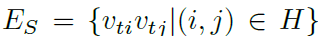
H는 naturally connected human body joints의 set입니다. second subset은 inter-frame edges를 contains하죠. 이는 consecutive frame에서 same joint를 connect합니다. 아래와 같이 표기합니다.

하나의 particular joint i에 대해 E_F에서 all edges는 time에 걸친 its trajectory를 represent합니다.
Spatial Graph Convolutional Neural Network
ST-GCN을 자세히 보기전에, 하나의 single frame에서의 graph CNN model을 먼저 본다고 합니다. 이 경우, t time에서 single frame에 대해, E_s(t) skeleton edges를 가진 N개의 joint nodes V_t가 있을 겁니다. feature maps나 2D natural images에 대한 convolution operation의 definition을 떠올려봅시다. convolution operation의 output feature map은 다시 2D grid 이죠. stride 1과 appropriate padding을 가지고, output feature maps는 input feature maps와 같은 size를 가질 수 있죠. 저자들은 following discussion에서 이 condition을 가정합니다. K x K 의 kernel size가진 convolution operator와 channels c개를 가진 input feature map f_in 주어지면, spatial loaction x에서 single channel에 대한 output value는 아래와 같이 쓰여질 수 있습니다.

sampling fuction p( Z^2 x Z^2 -> Z^2 ) 는 location x의 neighbors를 enumerate합니다. image convolution의 경우, p( x, h, w ) = x + p'( h, w )로 represented 될 수 있죠. weight function w ( z^2 -> R^c )는 dimension c의 sampled input feature vectors와 inner product를 computing하기 위한 c-dimension real space에서 weight vector를 provides 합니다. weight function은 input location x에 관련이 없습니다. 따라서 filter weights는 input image에 대해 모든 곳에서 shared 되죠. image domain에 대한 standard convolution은 p(x)에서 rectangular grid를 encoding하는 것에 의해 achieved 되죠.
graphs에 대한 convolution operation은 input features mape이 spatial graph V_t에 대해 resieds되는 cases 에서 formulation을 extending함으로써 defined 됩니다. 즉, f^t_in : V_t -> R^c 는 graph의 각 node에 대한 vector입니다. extension의 next step은 sampling function p와 weight function w를 redefine하는 겁니다.
Sampling function
image에 대해, sampling fuction p(h, w)는 ceter location x와 관련하여 neighboring pixels에 대해 difined 되죠. graphs에 대해 node v_ti의 neighbor set B(v_ti) = { v_tj | d(v_tj,v_ti) <= D }에 대해 sampling function을 정의합니다. 여기서 d(v_tj, v_ti) 는 v_tj 에서 v_ti까지의 minimum length를 표기합니다. 따라서 sampling fuction p : B(v_ti) -> V 는 아래와 같이 표기될 수 있죠.

D = 1을 사용했습니다. 즉, joint nodes의 1-neighbor set을 말하죠. D의 higher number는 다음 연구를 위해 놔두겠답니다.
Weight function
sampling function과 비교해서, weight function은 define 하는 것이 더 까다로운데요. 2D convolution에서 rigid grid는 center location 주위에 naturally exists하죠. 따라서 neighbor 한 pixels는 fixed spatial order를 가질 수 있죠. weight function은 그러면, spatial order를 따라 (c, K, K) dimensions의 tensor를 indexing 함으로써 implemented 될 수 있죠. general graph에 대해, implicit arrangement는 존재하지 않죠. 이 문제에 대한 solution은 다른 연구에서 제안 되었는데요. 해당 연구에서, order는 root node 주위의 neighbor graph에서 graph labeling process에 의해 defined되죠. 저자들 역시 이 idea를 따라 weight function을 construct했습니다. unique labeling을 모든 neighbor node에 부여하는 대신, joint node v_ti의 neighbor set B( v_ti ) set을 고정된 K 개의 subset으로 나눔으로써 simplify 하게 process했죠. 여기서 각 subset은 numeric label을 가집니다. 따라서 mapping l_ti : B(v_ti) -> { 0, ... , K-1 } 을 얻을 수 있고 이는 neighborhood에 대해 nodes를 its subset label로 map 하죠. weight function w ( v_ti, v_tj ) : B(v_ti) -> R^c는 (c, K) dimension의 tensor를 indexing 함으로써 얻을 수 있습니다. 식으로는 아래와 같이 쓸 수 있고요.

Spatial Graph Convolution
refined sampling function과 weight function을 가지고 Eq 1을 graph convolution 관점에서 다시 써보면 아래와 같죠.
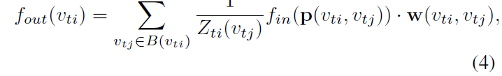
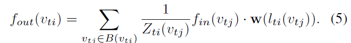
normalizing term Z_ti(v_ti) = | {v_tk | l_ti (v_tk) = l_ti(v_tj) } | 는 corresponding subset의 cardinality와 같습니다. 이 term은 output에 different subsets의 contributions을 balance하기 위해 추가됩니다. Eq 2와 Eq 3을 Eq 4에 대체하면 아래의 식을 얻을 수 있습니다.
만약 image를 regular 2D grid로 다룬다면 이 formulation이 standard 2D convolution과 resemble 할 수 있다는 것은 가치가 있죠. 예를 들어, 3 x 3 convolution operation을 resemble하기 위해, 3 x 3 grid 에 가운데 위치한 pixel에 대해 9 pixels의 neighbor를 가질 수 있죠. neighbor set은 9 개의 subset으로 나눠질수 있고, 각각 한 개의 pixcel을 가지게 되죠.
Spatial Temporal Modeling
formulated spatial graph CNN를 가지고, skeleton sequence 안에서 spatial temporal dynamics를 modeling하는 task로 발전시켜 본다고 하는데요. graph의 construction에서, graph의 temporal aspect는 consecutive frames에 걸쳐 same joints를 connecting함으로써 constructed 된다는 사실을 짚고 넘어갑시다. 이것은 spatial graph CNN을 spatial temporal domain으로 extend 하는 simple strategy를 define할 수 있게 해주죠. 즉, temporally connected joint를 include하는 neighborhood의 concept을 extend 하면 아래와 같이 쓸 수 있죠.

parameter gamma 는 temporal range를 control하는 데 , neighbor graph에서 included 되죠. gamma를 temporal kernel size 라고 부릅니다. spatial temporal graph에 대한 convolution operation을 complete하기 위해, sampling function이 필요하죠. sampling function은 spatial only case 그리고 weight function, 특별히, labeling map l_ST와 같죠. temporal axis가 well-ordered 되어 있기 때문에, v_ti에서 rooted 된 spatial temporal neghborhood에 대한 label map l_ST을 dirctly modifiy 하죠. 아래와 같이 말이죠.

l_ti (v_tj )는 v_ti에서 single frame case에 대한 label map입니다. 이런 방식으로 constructed spatial temporal graph에 대한 well-defined convolution operation을 가질 수 있죠.
Partition Strategies
spatial temporal graph convolution의 high-level formulation이 주어지면, label map l을 implement하는 partitioning strategy를 design 하는 것은 중요한데요. 이 연구에서, 저자들은 several partion strategies를 사용합니다. 간단하게 하기 위해, single frame에서의 case 만을 논의하는데 이는 Eq 7 을 사용해서 spatial-temporal domain으로 확장할 수 있기 때문이죠.
Uni-labeling
가장 simplest하고 straight forward partition strategy는 subset을 가지는 것이죠. 이는 whole neighbor set 이죠. 이런 strategy에서, every neighboring node에 대한 feature vectors는 same weight vector를 가진 inner product를 가질 수 있죠. 사실, 타 연구에서 도입한 propagation rule가 resemble하죠. single frame case에서 obvious drawback이 있는데, 이 strategy를 사용하는 것은 weight vector와 all neighboring nodes의 average feature vector 간에 inner product을 computing 하는 것과 동일하죠. skeleton sequence classification에 대해 suboptimal 하죠. local differential properties가 이 operation에서 lost될 수 있기 때문이죠. K = 1로 l_ti( v_tj ) = 0 을 가지고 있죠.
Distance partitioning
또 다른 natural partiioning strategy는 neighbor set을 root node v_ti 까지 nodes' distance d( dot, v_ti) 에 따라 나누는 겁니다. 이 연구에서는, D= 1로 set 했고, neighbor set은 두 개의 subset으로 나눠지죠. d = 0는 root node 자체를 뜻하고 neighbor nodes 를 remaining 하는 것은 d = 1인 subset 에 있죠. 따라서 두 개의 different weight vectors 를 가지게 됩니다 그리고 joints 간의 relative translation 와 같은 local differential properties를 modeling 할 수 있게 되죠. K = 2이고 l_ti( v_tj ) = d( v_tj, v_ti )입니다.
Spatial configuration partitioning
body skeleton이 spatially localized 되기 때문에, partitioning process에서 specific spatial configuration을 여전히 사용하는데요. neighbor set을 세 개의 subsets로 나눈는 strategy를 design 했습니다. 1) root node 2) centripetal group : skeleton의 gravity center에 root node보다 가까운 이는 neighboring nodes 들이죠 3) outherwise the centrifugal group ( 논문에 설명은 없지만, root node보다 skeleton의 gravity center 보다 먼 친구들 입니다. 이 내용은 전에 다른 논문에서 다뤘었죠. 물론 해당 논문이 더 이후의 논문이기 때문에 잘 다뤘던 것 같고 아마 2s-agcn에서 다뤘을 겁니다. ) skeleton에서 all joints의 average coordinate가 gravity center로 입니다. 이 strategy는 body aprts의 motions는 concentric 과 eccentric motions로 broadly 하게 categorized된다는 사실에 영감을 받았죠. 즉 아래와 같은 식을 구성하죠.
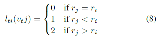
r_i는 gravity center 에서 joint i 까지의 average distance입니다.
three partitioning strategies의 Visualization Fig 3에서 볼 수 있죠.

저자들은 skeleton based action recognition experiments에서 proposed partioning strategies를 examine 할거라고 합니다. more advanced partitioning strategy는 capacity와 recognition performance 더 좋게 modeling하도록 만들거라 기대한다네요.
Learnable edge importance weighting
people이 actions을 performing 할때 joints가 group 안에서 move 함에도 불구하고, 하나의 joint는 multiple body parts에서 appear 할 수 있죠. 그러나, 이런 apperances는 these parts의 dynamics를 modeling하는데 있어 ifferent importance를 가지죠. 이런 관점에서, spatial temporal graph convolution의 모든 layer에 대해 learnable mask M을 추가하는 데요. 이 mask는 E_s안에서 각 spatial graph edge의 learned importance weight에 기반해 its neibhoring nodes에 node's feature의 contribution을 scale 할 겁니다. 실험적으로 이 mask를 adding 하는 것이 ST-GCN의 recognition performance를 imporve 할 수 있다는 것을 알아냈죠. 이 때문에 data dependent attention map을 가질 수 있다는 것 또한요.
Impelementing ST-GCN
graph-based convolution의 implementation은 2D 나 3D convolution처럼 stratightforward 하지 않죠. skeleton based action recognition을 위한 ST-GCN implementing에 대해 자세히 설명한다고 합니다.
기존 연구에 사용되었던 graph convolution의 유사한 implementation을 adopt한다고 하는데요. single frame에서 joint의 intra-body connections 는 adjacency matrix A 와 self-connections를 representing 하는 identity matrix I으로 represented 됩니다. single frame case에서, first partitioning strategy를 활용한 ST-GCN은 아래의 식으로 표현될 수 있죠


multiple output channels의 weight vectors는 wieght matrix W를 form하기 위해 stacked 됩니다. spatial temporal cases 하에서, ( C, V, T)의 tensor로서 input feature map을 represent할 수 있죠. graph convolution은 1 x Gamma standard 2D convolution 을 forming 함으로써 implemented 되고 resulting tensor와 normalized adjacency matrix을 second dimension에 대해 multiplies 하죠. 여기서 normalized adjacenecy matrix은 아래 처럼 표시됩니다.

multiple subsets을 가진 partitioning strategies를 위해, 이 implementation을 다시 한번 사용하죠. 그러나 adjacency matrix은 several matrixes A_j로 분해됩니다. 즉 아래의 식처럼 말이죠.

예를 들어, distance partitioning strategy에서, A_0 = I 이고 A_1 = A 이죠. Eq 9 는 아래의 식으로 transformed 됩니다.
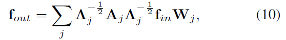

여기서 alpha = 0.001로 set하는 데 A_j에서 empty row를 피하기 위함이죠.
learnable edge importance weighthing 을 implement하는 것은 straightforward합니다. 각 adjacency matrix에 대해, learnable weight matrix M을 가진 adjacency matrix과 accompany합니다. 그리고 Eq 9 에서 A + I matrix과 Eq 10에서 A_j를 (A + I ) elemnet-wise product M 과 A_j elemnet-wise product M으로 대체합니다. mask M은 all-one matrix으로 initialized됩니다.
Network architecture and training
ST-GCN이 different nodes에 대해 weights를 share하기 때문에, different joints에 대한 input data consistent의 scale을 keep하는 것은 중요한데요. 실험에서, input skeletons을 data를 normalize하기 위해 batch normalization layer에 넣죠. ST-GCN model은 spatial temporal graph convolution operators의 9 layers로 구성되어 있는데요. 처음 3 개의 layer는 output을 위한 64개의 channels를 가지고 있죠. 뒤따라 나오는 세 개의 layer는 128개의 channels를 가지고 있고, 마지막 3 개의 layer는 256개의 channels를 가지고 있죠. 이 layers들은 9 개의 temporal kernel size를 가지고 있습니다. ST-GCN unit에 resnet mechanism이 applied되죠. overfitting을 피하기 위해 각 ST-GCN unit 후에 0.5 probability에서 features를 randomly하게 dropout합니다. 4-th와 7-th temporal convolution layers의 strides는 pooling layer로써 2로 set합니다. 그 후에, global pooling이 each sequence에 대해 256 dimension feature를 get한 resulting tensor에 대해 performed되죠. 마지막으로, 그들을 SoftMax classifier에 넣어주죠. model은 learning rate 0.01을 가진 SGD를 사용하여 learned되죠. 10 epoch 마다 0.1로 learning rate가 decay되죠. overfitting을 피하기 위해, dropout layers를 대체하는 두 종류의 augmentation 이 수행됩니다. 먼저, camera movement를 simulate하기 위해, random affine transformations가 all frames의 skeleton sequence에 대해 perform 되죠. first frame부터 last frame까지 few fixed angle, translation 그리고 scaling factor를 cnadidates로 select하고 그러고 난 다음 affine transformation을 generate하는 3 개의 factors의 two combinations 을 randomly하게 sampled하죠. 이 transformation은 intermediate frames에 대해 interpolated되는데 이는 playback 동안 view point를 smoothly하게 move하는 것과 같은 effect를 generate하죠. 이 augmentation을 random moving이라고 합니다. 두번째, training에서 original skelton sequence로부터 fragments를 randomly 하게 sample하고 test에서 all frames를 사용합니다. Global pooling은 network가 indefinite lenght를 가진 input sequences를 handle하게 해주죠.
여기까지 할게요
봐야할 부분은 다 챙기것 같네요


