원래 이렇게까지는 안하는데... csp를 구현해야할 부분이 있어서, 이번에는 논문 리뷰 후에 cspdarknet53 코드를 분석하는 시간을 가져볼게요..코드 분석은 다른 곳에 올릴 예정입니다. 최적화하는데 적용해야할 부분이 있어서 적용을 해보려고 합니다. 여튼 시작하시죠
Abstract
Neural networks는 object detection같은 vision tasks 에서 믿을 수 없는 결과를 달성하게하는 SOTA approaches를 가능하게 해왔죠. 그러나, 이런 굉장한 성공은 omputiation resources에 의존적이죠. 이는 advanced technology를 appreciating하는 cheap devices를 가진 사람들에게 방해 요소였고요. 이 논문에서 저자들은 Cross Stage Partial Network ( CSPNet )을 제안하는데 이전 연구들이 network architecture persepctive에서 heavy inference computations를 요구해왔던 문제를 완화시키죠. 저자들은 문제를 network optimization안에서 duplicate한 gradient information로 attribute하죠. 제안된 마지막 stage에서 computation을 20%까지 줄였습니다. 심지어 ImageNet dataset에 대해서는 accuracy가 더 우월하기도 하죠. SOTA approaches를 MSCOCO data에 대해 AP50 분야에서 SOTA approch를 앞지르기도 했습니다. CSPNet은 간단하게 구현가능하며 architectures에 cope 되기에 충분히 general하죠.
Introduction
Neural networks는 deeper 해지고 wider해질 때 특히 powerful 해지는 것을 보여왔는데요. neural networks의 확장은 엄청난 양의 계산을 야기했죠. object detection과 같은 heavy tasks를 많은 사람들이 이용하는 데 방해요소가 되어왔습니다. Light-weight computing이 점진적으로 주목을 받았는데 real-world applications가 short inference time을 small devices에 대해 요구했기 때문이죠. 이는 computer vision algroithms에 대해 심각한 challenge가 되었고요. depth-wise separable convolution tecniques는 Application-Specific Integrated Cirecuit( ASIC )와 같은 industrial IC design에는 경쟁력이 없습니다. 이 논문에서, 저자들은 RestNet, ResNeXt, DensnNet과 같은 SOAT approahes에 대해 computational burden에 대해 조사합니다. 저자들은 나아가 CPUs와 mobile CPUs 모두에 배포되는 mentioned networks를 가능하게 하는 efficient components를 개발하죠.
이 논문에서, 저자들은 Cross Stage Partial Network( CSPNet )을 도입합니다. CSPNet을 designing 하는 것의 주된 목적은 architecture가 computation 양을 줄이면서도 richer한 gradient combination을 achieve 하도록 하는 것이죠. 이 목적은 base layer의 feature map을 두 개의 part로 나눈다음 제안된 cross-stage에 따라 합쳐지는 방법으로써 가능합니다. 저자들의 main concept은 gradient flow가 different network paths를 따라 propagate하도록 하는 것인데요. 그를 위해 gradient flow를 나눈게 되죠. 이런 방식으로, 저자들은 propagated gradient information이 concatenation과 trasition steps를 switching함으로써 large correlation difference를 가질 수 있다는 것을 확인하였습니다. 게다가, CSPNet은 computation 양을 greatly하게 줄입니다. 그리고, inference speed와 accuracy역시 향상 시키죠. 이는 Fig 1에 설명되어 있습니다. proposed CSPNet-based object detector는 아래의 3가지 문제를 다룹니다.

1) Strengthening learning ability of a CNN
존재하는 CNN의 accuracy는 lightweightening이후에 greatly 하게 감소합니다. 그래서 저자들은 CNN's learning ability가 강화되길 바랐죠. 그래서 lightweightening이 되면서도 sufficient accuracy를 유지할 수 있게 되길 바랐습니다. 제안된 CSPNet은 ResNet, ResNeXt, 그리고 DenseNet에 쉽게 적용될 수 있습니다. CSPNet을 적용한 이후에, computation effort는 10%에서 20% 줄었고, original 성능을 뛰어넘습니다.
2) Removing computational bottlenecks
Too high한 computational bottleneck은 inference process가 complete해야하는 cycles를 더 많이 만들게 되죠. 그래서 저자들은 CNN의 각 layer에서 computation의 양이 공평하게 distribute할 수 있길 바랐고 computation unit의 utilization rate을 upgrade 할 수 있길 바랐죠. 그럼으로써 unnecessary energy consuption을 줄이고 싶었고요. proposed CSPNet은 computational bottlenects를 반으로 자릅니다. 저자들의 모델은 YOLOv3-based models에서 test할 때 80%의 computational bottleneck을 줄이죠.
3) Reducing memory costs
Dynamic Random-Access Memory( DRAM )의 wafer fabrcation cost는 매우 비쌉니다. 그리고 많은 공간을 차지하죠. 누군가 memory cost를 효과적으로 줄일수 있다면, 그 누군가는 ASIC의 cost를 엄청나게 줄일 수 있죠. 게다가 small area wafer는 edge computing devices에 다양하게 사용되죠. memory usage의 사용을 줄이는데 있어, 저자들은 cross-channel pooling을 적용합니다. 이는 feature maps를 feature pyramid generating process 중에 compress하죠. 이런방직으로 제안된 CSPNet은 memory usage를 75% 줄일 수 있었죠. 물론 feature pyramid를 생성할 때요.
CSPNet이 CNN의 learning capability를 증진시키기 때문에 저자들은 better accuracy를 위해 더 작은 모델을 사용합니다. 제안된 모델은 COCOAP50 에서 50%를 달성했고 109 fps를 달성했습니다. CSPNet은 memory traffic의 상당량을 cutdown 하기 때문에, 저자들의 방법은 다른 모델에서도 좋은 성능을 보이죠. 게다가 CSPNet이 computational bottleneck을 lower down 하기 때문에 Exact Fusion Model은 효과적으로 required memory bandwidth를 cutdown합니다.
Related work
CNN architectures design
ResNeXt는 cardinality가 width와 depth의 dimensions보다 더 효과적일 수 있다는 것을 처음 보여주었죠. DenseNet은 parameters의 수와 computations를 상당수 줄였는데 많은 수의 resuse feature를 적용하는 전략때문이었고요. DensNet은 preceding layres의 모든 output features를 concatenate하는데 이는 다음 input으로 사용되고, 이는 cardinality를 maximize하는 방법으로 고려될 수 있죠. SparseNet은 dense connection을 적용하는데, spaced connection은 parameter utilization을 improve할 수 있고 더 좋은 결과를 도출했죠. Wang et al.은 나아가 high cardinality와 sparse connection이 network의 learning ability를 impove할 수 있는지 gradient combination과 developed partial ResNet(PRN)의 concept으로 설명합니다. CNN의 inference speed를 올리기 위해, Ma et al. 은 4 개의 가이드라인을 도입했고 ShuffleNet-v2를 design했죠. Chao et al.은 loew memory traffic CNN을 제안했는데, Harmonic DenseNet이라 불리고 real DRAM trffic measurement로 DRAM traffic proportional의 approximation인 CIO ( Convolutional Input/Output ) metric을 제안했습니다.
Real-time object detector
가장 유명한 두 개의 real-time object detectors는 YOLOv3와 SSD 입니다. SSD에 기반해 LRF, RFBNet은 SOTA real-time object detection performance를 달성했죠. 최근, anchor-free based object detector가 object detection system의 main-stream이 되고 있습니다. Two object detector의 종류는 CenterNet과 CornerNet-Lite입니다. 그들은 모두 효율적으로 동작하죠. Real-time object detection을 위해, SSD-based Pelee, YOLOv3-based PRN 그리고 Light-Head RCNN-based ThunderNet은 object detection에 대해 훌륭한 performance를 보여줬죠.
Method
3.1 Cross Stage Partial Network
DensNet
Figure 2(a)는 DenseNet의 one-stage의 상세한 구조를 보여줍니다. 각 stage는 dense block를 포함하고 있고 trasition layer를 포함하고 있죠. 각 dense block은 k개의 dense layers로 구성되어 있습니다. i-th dense layer의 output은 i-th dense layer의 input과 concatenated 됩니다. 그리고 concatenated outcome은 i+1-th dense layer의 input이 되죠. 아래의 식은 위의 mechnism을 표현한 것이죠.

여기서 * 은 convolution operator를 나타냅니다. [x0,...]는 x0,... 를 concatenate했다는 것을 의미하고 w_i 와 x_i는 weights와 i-th dense layer의 output 을 각각 의미합니다.
만일 누군가 backpropagation algorithm 을 만든다면, wiehgt updating 의 equations은 아래와 같이 쓰여지겠죠.

여기서 f는 weight updating에 관한 function입니다. g_i는 i-th dense layer로 gradient propagated를 나타냅니다. 저자들은 많은 양의 gradient information이 updating weights를 위해 재사용된다는 것을 알아냈죠. 이거승ㄴ different dense layers는 반복적으로 copied gradient information을 학습하는 결과를 초래합니다.
Cross Stage Partial DenseNet
CSPDenseNet의 one-stage에 관한 architecture는 Figure 2 (b)에서 볼 수 있습니다. stage는 partial dense block과 aprtial transition layer로 구성되어 있습니다. partial dense block에서 stage에서 base layer의 feature maps는 channel x0 = [ x'0, x''0] 에 따라 두 부분으로 나눠집니다. x''0와 x'0 사이에서, 전자는 stage의 마지막 부분과 직접 연결되니다. 그리고 후자는 dense block을 통과하게 됩니다. 모든 steps는 partial transition layer가 포함되어 있으며 다음을 따릅니다: 먼저, dense layers의 output [x''0, x1, ... xk] 는 trainsition layer를 거칩니다. 다음으로 trainsition layer의 ouput은 x''0와 concatenated됩니다. 그리고 다른 transition layer를 거치죠. 그런 다음 output x_u를 생성합니다. feed-forward pass의 equations와 CSPDenseNet의 weight updating은 Equations 3과 4에서 각각 보여줍니다.
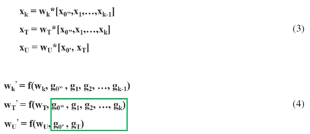
저자들은 dense layers로부터 gradients가 부분적으로 integrated 된다는 것을 발견했죠. 한편, featre map x'0는 dense layer를 거치지 않았고 부분적으로 integrated됩니다. updating weights를 위한 gradient information에 따르면, both sides는 other sides에 속한 duplicate gradient information을 포함하지 않습니다.
전반적으로 말해서, 제안된 CSPDenseNet은 DenseNet's feature reuse characteristics의 장점은 그대로 유지하면서도 동시에 gradient flow를 truncating함으로써 duplicate한 gradient information의 amout를 excessively하게 prevents하죠. 이 idea는 hierarchical feature fusion strategy를 designing 함으로써 realized되고 partial transition layer에서도 사용됩니다.
Partial Dense Block
partial dense blocks의 목적은 1)gradient path를 increase하는 겁니다: split and merge strategy를 통해, gradient paths의 수는 두배가 됩니다. cross-stage stratgy 때문에, 하나의 path는 concatenation을 위한 feature map copy를 사용함으로써 발생되는 disadvantages를 완화할 수 있죠; 2) 각 layer의 balance computation이 목적인데, DenseNet의 base layer에서 channel 수는 growth rate보다 훨씬 크죠. base layer channels가 original number의 절반만큼만을 차지하는 partial dense block에 대한 dense layer opration을 가지고 있기 때문에 computational bottleneck의 절반에 가깝게 효과적으로 solve할 수 있죠; 3) reduce memory traffic: DenseNet에서 dense block의 기본 feature map size는 w x h x c로 가정합니다. growth rate은 d인데 총 m개의 dense layer를 가지고 있죠. 그러면, dense block의 CIO는 ( c x m ) + ( ( m^2 + m ) x d ) / 2 이고 partial dense block의 CIO는 ( ( c x m ) + ( m^2 + m ) x d ) /2 입니다. m과 d는 c보다 작지만 partial dense block은 network의 memory traffic 에 대해 절반정도로 절약할 수 있습니다.
Partial Transition Layer
partial partial transition layers를 designing하는 것의 목적은 dradient combination의 difference를 maximize하는것 입니다. partial transition layer는 hierarchical feature fusion mechanism입니다. duplicate gradient information을 학습하는 것으로 부터 distinct layers를 prevent하는 gradient flow를 truncating 하는 전략을 사용한 것이죠. 저자들은 두 개의 CSPDensNet에 대한 variantions 을 design합니다. 이는 두 종류의 gradient flow truncating이 network의 learning ability에 영향을 미치는 정도를 보여주기 위함이죠. Fig 3(c)와 3(d)는 두 가지 다른 fusion 전략입니다. CSP ( fusion first ) 는 two parts에 의해 생성된 feature maps를 concatenat하는 것을 의미합니다. 그런다음 transition operation을 적용하죠. 이 전략이 적용된다면, 많은 양의 gradient information이 재사용될 겁니다. CSP ( fusion last ) 전략에서 처럼, dense block으로부터 output이 trainsition layer를 통과하게 되고 part 1로 부터 나온 feature map과 concatenation이 되죠. 만약 CSP( fusion last ) 전략을 취하게 되면, gradient information은 재사용되지 않을 텐데 이는 gradient flow가 truncated되기 때문이죠. 저자들이 4개의 architectures를 image classification을 위해 사용했는데, 해당 결과는 Figure 4에서 볼수 있죠.

CSP ( fusion last) 전략을 취하게되면, computation cost는 상당히 감소하지만 top-1 accuracy는 0.1% 감소하죠. 반면 Fusion frist 전약을 computation cost를 감소시키면서도 1.5%의 성능 감소를 가져옵니다. split and megre stratgy를 사용함으로써 저자들은 duplication의 possibility를 effectively하게 reduce할 수 있죠. Figure4의 결과로부터, repeated gradient information을 effectively하게 reduce할수 있다면 learning ability가 향상될 수 있다는 것은 명백하죠.
Apply CSPNet to Other Architectures
CSPNet은 ResNet과 ResNeXt에 쉽게 적용될 수 있죠. 이는 Figure 5에서 보여집니다.

feature channels의 반만이 Res(X)Blocks를 통과하기 때문에,bottleneck layer는 더 이상 필요없죠. 이는 FLoating-point OPerations( FLOPs )가 fixed 될떄 Memory Access Cost (MAC)의 이론적인 lower bound를 만들죠.
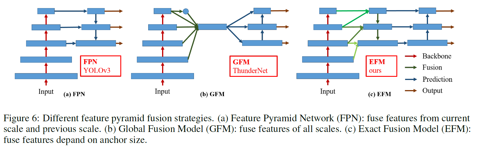
Exact Fusion Model
Looking Exactly to predict perfectly
저자들은 EFM을 제안하는데 각 anchor에 대해 적절한 FoV ( Field of View )를 captures하죠. 이는 one-stage object detector의 accuracy를 강화하고요. segmentation task에 대해 pixel-level labels는 global information을 포함하고 있지 않기 때문에, 더 나은 information retrieval을 위해 larger patches를 고려하는 것은 더 선호되죠. 그러나 image classification이나 object detection과 같은 tasks에 대해, critical information은 image-level과 bounding box-level labels로부터 관찰될 떄 obscure 할 수 있습니다. Li et al 은 CNN은 image-level labels로 부터 학습할 때 distracted 될 수 있다는 것을 발견했고 two-stage object detectors가 one-stage object detectors를 뛰어넘는 주요한 요인이라고 결론지었죠.
Aggregate Feature Pyramid
제안된 EFM는 initial feature pyramid를 더잘 aggregate할 수 있죠. EFM은 YOLOv3에 기반합니다. 이전 each ground truth object에 정확하게 하나의 bounding-box를 할당하죠. 각 groundtruth bounding box는 하나의 anchor box에 해당하는데 해당 anchor box는 threshold IoU를 넘는 박스들이죠. anchor box의 size가 grid cell의 FoV와 equivalent하다면 s-th scale의 gird cells에 대해, 해당하는 bounding box는 (s-1)-th scale에 의해 lower bounded 될겁니다. 그리고 (s+1)-th scale에 의해 upper bounded될 것고요, 따라서 EFM 은 3개의 scales로 부터 features를 assembles합니다.
Balance Computation
feature pyramid로부터 concatenated feature maps가 enormous하기 때문에, 많은 memory와 computation cost 가 필요하죠. 이 문제를 해결하기 위해 Maxout technique을 feature maps를 compress하는데 도입합니다.
마지막 그림은 실험에서 사용된 그림인데 참고용로 보시면 될 것 같네요
실험 부분은 생략하겠습니다.


