안녕하세요. WH입니다
오랜만에 글을 쓰네요
이것저것 일이 많아서요
오늘은 optical flow에 관한 논문입니다.
이걸 왜 하냐,
optical flow는 spatial information을 얻는 하나의 방법이죠
다음 프로젝트에 필요하기 때문에
정리하게 되었습니다.
원래는 opencv의 opticalflow를 활용하면 되지만
이번 하드웨어는 opencv를 지원하지 않거든요.
C++로 구현하느니..모델을 쓰자는 생각에서 시작합니다.
18년 논문이긴 하지만 어쩌겠어요.
하드웨어가 기술을 못따라 가네요..여튼
함께보시죠
Abstract
저자들은 opitcal flow를 위한 compact하지만 effective CNN model인 PWC-Net을 제안합니다. PWC-Net은 간단하면서도 잘 설계된 원칙에 따라 designed 되었다고 하는데요. 그 것은 pyramidal processing, warping, 그리고 cost volume의 사용입니다. learnable feature pyramid에 Cast된 PWC-Net은 second image의 CNN features를 wrap한 current optical flow estimation을 사용합니다. 그런 다음 warped features와 cost volume을 construct하는 first image의 features 사용하죠. 이는 optical flow을 estimate하는 CNN에 의해 처리되죠. PWC-Net은 FlowNet2 model보다 학습하기 쉬우며 17배 작은 size를 가지고 있죠. 게대가 성능 또한 당시 기준으로 가장 좋았다고 하네요.
Introduction
Optical flow estimation는 core computer vision problem이죠. 그리고 많은 application이 있죠. action recogntion, autonomous driving, video editing 이 예가 되겠네요. 십 수년간 연구의 노력들이 challenging benchmarks에서 인상적인 성능을 야기했죠. Most top-performing methods는 energy minimization approach가 적용되었죠. 이는 Horn and Schunck에 의해 소개되었고요. 그러지만, complex energy function을 optimizing하는 것은 real-time applications에서 computationally expensive 합니다.
하나의 promising approach는 fast, scalable, 그리고 end-to-end trainable CNN framework을 적용하는 것이죠. 최근 수년간 computer vision 분야에서 엄청난 진보가 있기에 가능하죠. high-level vision tasks에서 deep learning의 successes에 영감을 얻어, Dosovitskiy는 optical flow를 위한 two CNN model을 제안합니다. 그것은 FlowNetS와 FlowNetC 이죠. 그리고 paradigm shift를 도입했죠. 그들의 work은 U-Net CNN architecture를 사용하여 raw images로 부터 optical flow를 직접 estimating의 실현 가능성을 보여줬죠. 그들의 성능은 SOTA보다 낮았지만, FlowNetS와 FlowNetC models는 real-time methods 중에 best한 것이죠.
최근, Ilg 는 몇 개의 FlowNetC와 FlowNetS를 large model에 쌓았죠. 그리고 FlowNet2라고 불렀습니다. FlowNet2는 성능면에서 SOTA method와 비슷했지만 훨씬 빨랐습니다. 그렇지만 large model은 over-fitting problem이 발생하기 쉽고, 결과적으로 FlowNet2의 subnetworks가 연속적으로 trained 되야만 하죠. 게다가 FlowNet2는 640MB의 memory footprint가 필요합니다. 이는 mobile이나 embedded devices에 적합하지 않죠.
SpyNet은 model size issue를 다뤘습니다. 두 개의 classical optical flow estimation principles를 deep learning과 결합하는 방식으로 말이죠. SpyNet은 spatial pyramid network를 가용하고 second image를 initial flow를 사용하는 first ones로 warp 합니다. first 와 warped images 사이에 motion은 대게 작죠. 따라서 SpyNet은 단지 two images로 부터 motion을 estimate하는 small network이 필요할 뿐이죠. SpyNet은 FlowNetC와 비슷한 성능을 보이지만 FlowNetS와 FlowNet2 보다는 좋지 않죠. FlowNet2와 SpyNet은 accuracy와 model size의 trade-off 관계를 명확하게 보여줍니다.
optical flow를 위한 CNN model의 size를 줄이면서 accuracy는 증가시키는 것이 가능할까요? 이론적으로, model size와 accuracy 간의 trade-off는 general machine learning algoriths에 대한 fundamental limit을 부과하죠. 그러나, 저자들은 deep learning과 domain knowledge를 combining이 두 가지 goals를 동시에 성취할 수 있다는 것을 밝힙니다.
SpyNet은 classical principles를 CNN과 combining에 대한 잠재성을 보여주죠. 하지만, 저자들은 FlowNetS와 FlowNet2의 performance gap은 classical principles의 partial use 때문이라고 주장합니다. 먼저, traditional optical flow methods는 종종 shadows나 lighting changes에 불변하는 feature를 extract하는 raw images를 pre-process하죠. 게다가, stero matching의 special case에서 cost volume은 raw images나 features의 보다 disparity의 더 discriminative representation하죠. full cost volume을 constructing 은 real-time optical flow estimation에 대해 computationally prohibitive하지만, 이 연구는 search range를 each pyramid level로 제한함으로써 partial cost volume을 construct하죠. 저자들은 large displacement flow를 estimate하는 wraping layer를 사용하여 different pyramid levles를 link할 수 있습니다.
저자들의 network는 PWC-Net이라고 불리고 이 간단하고 잘 설계된 principles를 모두 사용하여 만들었죠. 이는 optical flow를 위해 존재하는 CNN models들을 accuracy와 size 에 대해 넘어서는 significant improvement를 이끌었죠. 이 논문이 쓰여지는 시기에, PWC-Net은 출간된 flow methods를 모두 뛰어넘었습니다. 게다가 PWC-Net은 FlowNet2에 비해 17배 작고 2배 빠르죠. 또한 SpyNet과 FlowNet2보다 학습시키기 쉽고 약 35 FPS가 나오죠.
Previous Work
Variational approach
Horn and Schunck는 brightness constancy와 energy function을 이용한 spatial smoothness assumption을 coupling함으로써 optical flow에 대한 variational approach를 개척했죠. Black 과 Anandan은 outliers를 다루는 robust framework을 도입했고요. ( brightness inconstancy 와 spatial discontinuities ) full search를 수행하기에 computationally impractical 하기 때문에, warping-based approach가 적용됬죠. Brox는 이론적으로 warping-based estimation process를 증명했습니다. Sun 은 models, optimization. 그리고 Horn과 Schunck에 의해 제안된 models를 위한 implementation details를 review하고 motion details를 recover하는 non-local term을 제안합니다. coarse-to-fine, variational approach는 optical flow에서 가장 popular framework이죠. 그러나, 그것은 complex optimization problems를 solving하는 것을 요구하죠. 그리고 real-time applications에 대해 computationally expensive하죠.
coarse-to-fine approach의 하나의 난제는 coarse levels에서 사라지는 small and fast moving objects죠. 이 문제를 address하기 위해, Brox 와 Malik는feature matching을 variational framework에 embed했죠. 이는 이어 나오는 연구에서 더 향상되었고요. 특별히 EpicFlow method는 sparse mathces를 dense optical flow에 효과적으로 interpolate 할 수 있죠. 그리고 post-processing method로 널리 사용되고요. Zweig 와 Wolf는 sparese-to-dense interpolation을 위한 CNN을 사용했죠. 그리고 EpicFlow를 넘어서는 consistent improvenment를 얻었습니다.
Most top-performing methods는 CNN을 그들의 system의 구성요소로 사용합니다. 예를 들면, DCFlow는 full cost volum을 construct하는 CNN features를 학습합니다. 그리고 optical flow를 estimate하는 sophisticated post-procesiing techniques를 사용하죠. EpicFlow를 포함하죠. 그 다음 좋은 method는 FlowFieldsCNN 인데요, 이는 sparse matching을 위한 CNN feature를 학습하죠. EpicFlow에 의해 matches를 densifies 하죠. 세 번째 방법은 MRFlow인데요. 이는 scene을 rigid와 non-rigid regions으로 분류하는 CNN을 사용합니다. 그리고 rigid region에 대해 plane + parallax formulation을 사용하여 geometry와 camera motion을 estimate하죠. 그러나, 이들 중에는 real-time 이나 end-to-end trainable에 대한 것은 없죠.
Ealry work on learning optical flow
Simoncelli 와 Adelson은 optical flow를 위한 data matching errors를 연구했죠. Freeman은 syntetic blob world examples를 사용해서 image motion을 위한 MRF model의 parameter를 연구했고요. Roth와 Black은 depth maps으로 부터의 sequence generated를 사용해 optical flow의 spatial statics를 연구했죠. Sun은 optical flow를 위한 full model을 연구했습니다. 그러나 연구는 few training sequence로 제한되었죠. Li 와 Huttenlocker는 Black 과 Anandan method에 대한 parameters를 tune하는 stochastic optimization을 사용했죠. 그러나 학습된 parameters의 수가 제한되었죠. Wulff 와 Black은 real movies에서 GPUFlow에 의해 추정된 optical flow의 PCA motion basis를 연구했죠. 그들의 method는 빠르지만 over-smoothed flow를 생성합니다.
Recent Work on learining optical flow
high-level vision task에서 CNN의 성공에 영감을 얻어, Dosovitskiy는 U-Net denoising autoencoder에 기반한 optical flow를 추정하기 위한 두 개의 CNN networks를 construct합니다. FlowNetS와 FlowNetC이죠. 이 networks들은 large synthetic FlyingChairs dataset에서 pre-trained 되었습니다. 그러나 놀랍게도 Sintel dataset에서 빠르게 움직이는 물체의 motion을 capture할 수 있죠. 그러나 network의 raw output은 smooth backgruond regions에서 large errors를 포함하죠. 그리고 variational refinement를 요구하죠. Mayer은 FlowNet architecture를 disparty와 scene flow estimation에 적용합니다. Ilg는 기본 FlowNet models를 쌓아 크게 만들었죠. 이 model이 FlowNet2입니다. 이는 Sintel benchmark에서 SOTA에 비견되는 성능을 보여줍니다. Ranjan과 Black은 compact spatial pyramid network을 개발했죠. SpyNet이라고 불립니다. SpyNet은 FlowNetC model 과 유사한 성능을 달성했죠. 그렇지만 SOTA는 아니었죠.
또 다른 흥미로운 연구줄기는 unsupervised learning approach인데요. Memisevic과 Hinton은 unsupervised way로 image transformation을 학습하는 gated restricted Boltzmann machine을 제안하죠. Long은 frames를 interpolating함으로써 optical flow를 위한 CNN model을 연구했죠. Yu는 spatial smoothness term에 data constancy term을 결합한 loss term을 minimize하는 models를 train했죠. labeled training data를 가진 dataset에서 supervised approaches에 비해 inferior하긴 하지만, existing unsupervised methods는 unlabeled data에서 CNN model을 학습하는 데 사용할 수 있죠.
Cost volum
cost volume은 pixel과 next frame에서 그에 해당하는 pixels을 associating을 위한 data matching cost를 stores하죠. 그것의 computation과 processing은 stereo matching을 위한 standard components죠. optical flow의 special case입니다. Recent methods는 optical flow를 위한 cost volume processing를 investigate하죠. 모두가 single scale에서 full cost voulme을 build합니다. 이는 computationally expensive하고 memory intensive하죠. 반면에, 저자들의 연구는 partial cost volume를 multiple pyramid levels에서 constructing 은 effective와 efficient models로 이끈다는 것을 보여줍니다.
Datasets
많은 다른 vision task와 다르게, real-world sequence에서 ground truth optical flow를 얻는 것은 extremely difficult하죠. optical flow 에 대한 Early work은 synthetic datasets에 의존하죠. Yosemite 가 예가 되겠네요. Methods는 synthetic data에 over-fit되어 real data에서 잘 작동하지 않죠. Baker는 ground truth를 얻기위해 controlled lab enviromnment에서 ambient 와 UV lights 에서 real sequence를 capture했죠. 그러나 해당 approach는 outdoor scenes에서 동작하지 않죠. Liu는 natural video sequences를 위한 ground truth motion을 얻은 human annotiations 를 사용합니다. 그러나 labeling process는 time-consuming하죠.
KITTI와 Sintel은 currently the most challenging이죠. 그리고 optical flow를 위한 benchmarks로 널리 이용되죠. KITTI ㅠbenchmark는 autonomous driving applications를 targeted하죠. 그리고 semi-dense ground truth는 LIDAR을 사용해 collected 되죠. 2012 set은 static scenes로만 구성됩니다. 2015 set은 human annotations를 통해 dynamic scenes로 확장되죠. 그리고 2015 set은 existing methods에 more challenging한데요. large motion, severe illumination changes, 그리고 occlusions 때문이죠. Sintel benchmark는 two pass를 가지는 open source graphics movie Sintel ( clean과 final )를 활용해 만들어졌죠. final pass는 strong atmospheric effects, motion blur, 그리고 camera noise가 포함되어있죠. 이는 현존하는 모델에게 문제를 야기하죠. top-performing methods는 traditional techniques에 heavily 의존하죠. classical principles를 network architectur로 embedding하면서, 저자들은 fully end-to-end methond가 모든 published methods를 KITTI 2015와 Sintel final pass benchmarks에서 뛰어넘을 수 있음을 보여줍니다.
CNN models for dense prediction tasks in vision
denoising autoencoder는 computer vision에서 dense prediction tasks를 위해 흔히 사용되는데요. 특히 encoder와 decoder간에 skip connections를 가지고 있죠. 최근 연구는 dilated convolution layers가 contextual information을 더 잘 exploit할 수 있고 semantic segmentation에 대한 details를 refine할 수 있다는 것을 보여주는데요. 여기 저자들은 optical flow를 위한 contextual information을 integrate하기 위해 dilated convolutions를 사용했다고 합니다. 그리고 moderate performance improvement를 얻었다고 합니다. DenseNet architecture는 feedforward fashion에서 each layer를 every other layer에 직접연결합니다. 그리고 traditional CNN layers보다 image classification task에서 더 accurate하고 쉽게 학습된다는 것을 보여주죠. 저자들은 dense optical flow prediction을 위해 이 idea를 test했다고 합니다.
Approach

Figure 3은 PWC-Net의 key componets를 요약하죠. 그리고 traditional coarse-to-fine approach와 나란히 비교합니다. 먼저, raw image는 shadow와 lighting changes에 variant하기 때문에, 저자들은 learnable feature pyramids를 가진 fixed image pyramid로 대체했죠. 두 번째, 저자들은 traditional approach로부터 warping operation을 large motion을 추정하기는 저자들의 network에서 layer로써 채택했습니다. 세 번째, cost volume은 raw images보다 optical flow의 더 차별적인representation 인데요. 저자들의 network는 cost volume을 construct하는 layer를 가지고 있죠. 이는 flow를 추청하는 CNN layers에 의해 처리되죠. warping과 cost volume layers는 learnable parameter가 없고 model size를 줄입니다. 마지막으로 traditional methos를 통한 common practice는 contextual information을 사용해서 optical flow를 post-process하는 것입니다. median filtering과 bilateral filtering 같은 것들이 있겠죠. PWC-Net은 optical flow를 refine한 contextual information을 exploit하는 context network를 사용합니다. energy minimization과 비교하면 wraping, cost volume 그리고 CNN layers가 computationally light하죠.
다음, 저자들은 main ideas를 설명한다고 합니다. each components에 대해 말이죠. pyramid feature extractor, optical flow estimator, 그리고 context networks를 포함해서 말이죠.
Feature pyramid extractor
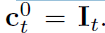
I_1과 I_2 두 개의 input images가 주어지면, 저자들은 feature represestations의 L-level pyramid 생성합니다. bottom(zeroth) level 이 input images로 존재할 경우 아래와 같이 표시합니다.
l th layer에서 feature representation을 생성하기 위해, 저자들은 l-1 th pyramid level에서 features를 downsample하는 convolutional filters의 layers를 사용합니다. 처음부터 여섯 번째 levels까지, features의 channels는 각각 16, 32, 64, 96, 128, 196 입니다.
Warping layer
l th level에서, 저자들은 second image를 first image로 warp하는데요. l+1th level로 부터 x2 upsampled flow를 사용합니다. 식은 아래와 같죠

여기서 x는 pixel index입니다. upsampled flow up_2(w^l+1)은 top level에서 zero로 set합니다. 저자들은 warping operation을 구현하는 bilinear interpolation 을 사용하고 input CNN features에 gradients를 compute하죠. backpropagation을 위한 flow는 기존 연구를 참고합니다. non-translational motion에 대해, warping은 몇몇 gemetric distortions을 compensate 할 수 있죠. 그리고 image pathches를 right scale에 넣어줄 수 있습니다.
Cost volume layer
다음, 저자들은 pixel이 다음 frame에서 그에 해당하는 pixels와 associating을 위한 matching costs를 저장하는 cost volume을 construct하는 features를 사용하는데요. 저자들은 matching cost를 first image와 second image warped features 간의 correlation으로 정의합니다. 식으로 표현하면 아래와 같죠
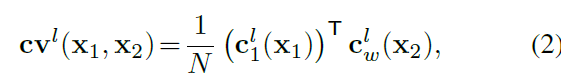
여기서 T는 transpose operator입니다. N은 column vector C_1^l(x_1)의 length 입니다. L-level pyramid setting에 대해, 저자들은 d pixels의 limited range를 가진 partial cost volume을 계산만 하면 되죠. limited range의 예시는 아래와 같습니다
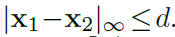
top level 에서 one-pixel motion은 full resolution images에서 2^(L-1) pixels에 해당합니다. 따라서 저자들은 d를 작게 설정할 수 있죠. 3D cost volume은 d^2 x H^l x W^l입니다. 여기서 H^l과 W^l은 l th pyramid level에서의 height와 width를 표기하죠.
Optical flow estimator
이 estimator는 multi-layer CNN인데요. input은 cost volume, 첫 번째 images의 features 그리고 upsampled optical flow 입니다. 그리고 이것의 output은 l th level에서의 flow w^l이죠. 각 convolutional layers에서 feature channels의 numbers는 각각 128, 128, 96, 64, 32 입니다. all pyramid levels에서 고정된채 유지되죠. different levels에서 이 estimators는 그들의 own parameters를 가집니다. same parameters를 sharing하지 않는다는 말이죠. 이 estimation process는 l_0까지 반복됩니다.
이 estimatro architecture는 DensNet connections를 가지고 enhanced되는데요. every convolutional layer에 inputs는 이전 layer에 대한 input과 output들입니다. DenseNet은 traditional layers에 비해 더 직접적인 연결을 가집니다. 그리고 image classification에서 주요한 improvement를 야기하죠. 저자들은 이 아이디어를 dense flow prediction에 대해 test합니다.
Context network
Traditional flow methods는 flow를 post-process하는 contextual information을 사용하는데요. 따라서 저자들은 desired pyramid level에서 각 output unit의 receptive field size를 효과적으로 enlarge하는 sub-network을 사용합니다. 이를 context network라고 부릅니다. 이는 estimated flow와 optical flow estimator로부터 second last layer의 features를 받아 refined flow를 출력합니다.
context network은 feed-forward CNN 인데요. 설계는 dilated convolutions에 기반합니다. 7 개의 convolutional layers로 구성되어 있습니다. 각 convolutional layer에 대한 spatial kernel은 3 x 3입니다. 이 layers는 different dilation constants를 가지는 데요. dilation constant k 를 가지는 convolutional layer는 layer에서 filter에 대한 input unit이 layer에서 fileter에 대한 다른 input unit과 수직, 수평 방향으로 떨어진 k개의 unit임을 의미합니다. large dilation을 가진 Convolutional layers는 large computational burden의 발생 없이 각 output의 receptive field를 확대합니다. bottomp에서 top까지 dilation constants는 1,2,4,8,16,1,1 입니다.
Training loss
세타를 learnable parameters의 set이라고 합시다. feature pyramid extractor와 optical flow estimator를 포함하죠. w_세타^l 은 flow field로 표기합니다. W_GT^l 은 supervision signal에 해당하죠. 저자들은 multi-scale training loss 를 사용합니다. 식은 아래와 같죠

| |_2는 vetor의 L2 norm을 계산하죠. 두 번째 term은 regularize parameter 입니다. fine-tuning에 대해, 아래의 training loss를 사용합니다 (lpq_loss 입니다 )

| |는 L1 norm을 나타냅니다. q <1 으면 less penalrty를 outliers에 부여합니다. 엡실론은 매우 작은 상수이고요
오늘은 여기까지 하겠습니다.
그 동안 코로나도 걸리고,
돌아와서 일도 바쁘고,
하드웨어 맞춰서 구현해야하는 일이 많아서
좀 힘들었네요.
옛날 framework을 빌드하느라 고생도 많이 했구요
여튼 여기까지할게요


