논문을 읽은 때는 항상 즐겁죠
적용할 때는 다른 이야기지만요
왜 보냐
아마도 st-gcn 논문을 볼 때
gcn에서 이를 언급했던 것이라 정리 차원에서 봅니다.
CenterNet에서도 나왔죠.
upsample layer 앞에서 deformable Convolution layer를 썻다고 했으니까요.
그게 뭐길래, 그죠? 시작합니다.
Abstract
CNNs는 본질적으로 geometric transformations를 model하도록 제한되어 있는데, 이는 their building modules에서 fixed geometric structures 때문이죠. 이 논문에서, 저자들은 새로운 두 가지 modules를 도입하죠. 이 modules는 CNNs의 transformation modeling capability를 enhance 하죠. deformable convolution 과 deformable RoI pooling이죠. 두 modules 모두 additional offsets를 가진 modules에서 spatial sampling locations를 augmenting 하는 것과 target tasks로부터 offsets를 learning 하는 것을 기본 idea로 하죠. 물론 additional supervision은 없습니다. deformable convolutional networks가 나오면, new modules는 기존 CNNs 에 exisiting 하는 plain counterparts를 readily하게 replace할 수 있죠. 그리고 standard back-propagation으로 end-to-end하게 trained 될 수 있습니다.
Introduction
visual recognition에서 key challenge는 어떻게 geometric variations를 accommodate 하거나 object scale, pose, viewpoint, 그리고 part deformation에서 geometric transformation을 model 할지 입니다. 일반적으로는 두 가지 방법이 있습니다. 처음 방법은 sufficient desired variations를 가진 training datasets를 build하는 겁니다. 이는 existing data samples를 augmenting 것으로 실현되죠. 가령 affine transformation 등이 있죠. Robust representations는 data로 부터 learned 될 수 있죠. 그러나 대게는 expensive한 training 과 complex model parameter를 대가로 치르죠. 두 번째는, transformation-invariant features와 algorithms를 사용하는 겁니다. 이 category는 잘 알려진 techniques가 포함되죠. 가령 SIFT ( scale invariant feature transform )과 object detection paradigm 기반의 sliding window 가 있겠죠.
그러나 위 방법들에는 두 가지 drawbacks가 있죠. 먼저, geometric transformations는 fixed와 known을 가정하죠. 그런 prior knowledges는 data를 augment하는데 사용되죠. 그리고 features와 algorithms을 designs합니다. 이 assumption은 unknown geometric transformations를 prossessing하는 new tasks로 generalization을 prevents하죠. 이는 적절하게 modeled된 것이 아니고요. 두 번쨰, invariant features와 algorithms의 hand-crafted design은 어려울 수 있고, overly complex transformations에 대해 infeasible할 수 있죠. 그것이 심지어 잘아는 것이라 할지라도요.
최근, CNNs는 visual recognition tasks에 대해 굉장한 성과를 달성해왔죠. 가령 image classification, semantic segmentation, 그리고 object detection 같은 task에서 말이죠. 그럼에도 불구하고, 그들은 두 가지 drawbacks를 share하죠. geometric transformations를 modeling하는 their cpapbility가 extensive data augmentation, large model capacity 그리고 some hand-crafted modules( 가령 small translation-invariance를 위한 max-pooling ) 로부터 나온다는 거죠.
요약하면, CNNs는 본질적으로 large, unknown transformations를 model하는데 한계가 있죠. limitation은 CNN modules의 fixed geometric sturctures로 부터 기인하고요: convolution unit은 input feature map을 fixed location에서 sample합니다; pooling layer는 fixed ratio에서 spatial resolution을 reduce하고요; RoI pooling layer는 fixed spatial bins로 RoI를 separates하죠. geometric transformations를 다루는 internal mechanisms가 lack하죠. 이는 moticeable problems를 야기합니다. 하나의 예를 들면, same CNN layer에서 all activation units의 receptive field sizes는 같죠. 이는 sematics 를 spatial locations에 걸쳐 encode하는 high level CNN layer에 대해 undesirable합니다.왜냐하면 different locations는 different scales나 deformation을 가진 objects로 correspond하기 때문에, scales 나 receptive field size에 대해 adaptive determination이 fine localization을 활용하는 visual recognition에 대해 desirable하죠. 또 다른 예시로, object detection은 significant하고 rapid progress를 보여온 반면, all approaches는 primitive bounding box based feature extraction에 여전히 의존적이죠. 이는 분명히 sub-optimal입니다. 특히 non-rigid objects에 대해서는 더 그렇죠.
이 연구에서, 저자들은 두 개의 modules를 도입하는데, geometric transformations의 CNN's capability를 greatly하게 강화하죠. 먼저 deformable convolution입니다. 여기에는 standard convolution에서 regular grid sampling locations로의 2D offsets가 추가됩니다. 그것은 sampling grid의 free form deformation을 가능하게 하죠. 이는 Figure 1에 설명되어 있습니다.

the offsets는adiitional convolutional layer를 통해 preceding feature maps로부터 learned 되죠. 따라서, deformation은 local, dense 그리고 adaptive한 방법으로 input features에 의해 conditioned됩니다.
두 번째는 deformable RoI pooling 입니다. 이는 previous RoI pooling의 regular bin partition 에서 each bin position에 offsets를 추가하죠. 유사하게, offsets는 preceding feature maps와 RoIs로부터 learned 됩니다. 이는 different shapes를 가진 objects에 대해 adaptive part localization을 가능하게 하고요.
두 modules 모두 light weight 입니다. 그들은 offset learning을 위해 small amount of parameters와 computation을 추가하죠. 그들은 deep CNNs에서 plain counterparts를 readily하게 replace할 수 있죠. 그리고 standard backpropagation을 활용해 end-to-end로 쉽게 trained 될 수 있죠. CNNs의 resulting은 deformable convolutional networks 나 deformable ConNets라고 불립니다.
저자들의 approach는 spatial transform networks 그리고 deformable part models와 유사한 high level spirit을 공유합니다. 그들은 모두 internal transformation parameters를 가지고 data로부터 purely하게 그런 parameters를 learn합니다. deformable ConvNets에서 key difference는 deformable ConvNets는 simple, efficient, deep and end-to-end한 방식으로 dense spatial transformations를 다룬다는 거죠. Section 3.1에서, 저자들은 저자들의 연구와 기존 연구의 관계에 대해 자세히 다루고 우월성을 분석한다고 합니다.
Deformable Convolutional Networks
CNNs에서 feature maps와 convolution은 3D입니다. deformable convolution과 RoI pooling modules는 2D spatial domain에서 operate하죠. operation은 channel dimension을 따라 같습니다. generality의 loss 없이, modules는 notation clarity를 위해 2D로 descirbed 됩니다. 3D로 extension은 직관적이죠.
Deformable Convolution
2D convolution은 two steps로 구성됩니다 : 1) input feature map x에 걸쳐 regular grid R을 사용하여 sampling하고; 2) w로 weighted 된 sampled values의 summation 합니다. grid R은 receptive field size와 dilation을 정의합니다. 예를 들면, 아래와 같이 정의된 R을 보죠

위의 R은 dilation1을 가진 3 x 3 kernel 입니다.
output feature map y에 대해 각 location p_0 를 위해, 저자들은 아래의 식을 가집니다.

sampling은 irregular하고 offset locations ( p_n + delta p_n )에서 됩니다. offset delta p_n이 typically fractional하기 때문에, Eq. (2)는 bilinear interpolataion을 통해 아래와 같이 나타낼 수 있죠

p 는 arbitrary( fractional ) location을 표기합니다 ( p = p_0 + p_n + delta p_n ). q 는 feature map x에서 all integral spatial locations를 enumerates 합니다. 그리고 G ( )는 bilinear interpolation kernel을 나타내죠. G는 two dimensional입니다. 이는 두 개의 one dimensional kernels로 나눠질 수 있고 아래와 같이 나옵니다.

g( a, b ) = max( 0, 1 - | a - b | ) 입니다. Eq (3) 은 G ( q, p )가 few q에 대해 non-zero 이기 때문에, 계산하기에 빠릅니다.

Figure 2에서 설명되어 있는 것처럼, offsets는 same input feature map에 걸처 convolutional layer를 applying 하는 것으로 obtained 될 수 있죠. convolution kernel은 current convolutional layer가 가지고 있는 것과 동일한 spatial resoltion과 dilation을 가지고 있습니다. ( 예를 들면, Figure2에서 dilation 1을 가진 3 x 3 을 들수 있죠 ). output offset fields는 input feature map과 동일한 spatial resolution을 가집니다. channel dimension 2N은 N 개의 2D offset에 해당하죠. training 동안, output features와 offsets를 generating을 위한 convolutional kernels 는 동시에 학습됩니다. offsets를 learn하기 위해, gradients는 Eq3과 Eq4에서 bilinear operations을 통해 backpropagated 됩니다.
Deformable RoI Pooling
RoI pooling은 object detection methods 기반 all region proposal에 사용됩니다. RoI pooling은 arbitrary size의 input rectangular region을 fixed size features로 converts 하죠.
RoI Pooling
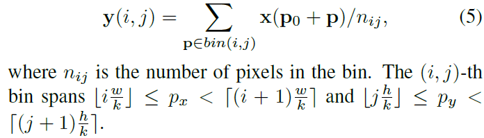
input feature map x 와 w x h size, top-left corner p_0의 RoI가 주어지면, RoI pooling은 RoI를 k x k로 ( k는 free parameter ) bins로 나뉩니다. 그리고 k x k feature map y를 outputs 하죠. ( i, j )-th bin ( 0 <= i, j < k )에 대해, 저자들은 아래의 식을 가집니다.
Eq 2와 유사하게, deformable RoI pooling에서 offsets 가 spatial binning positions에 추가 됩니다. Eq 5는 아래 처럼 바뀌죠.
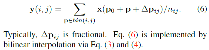
Figure 3은 offests를 obtain하는 방법에 대해 설명합니다.
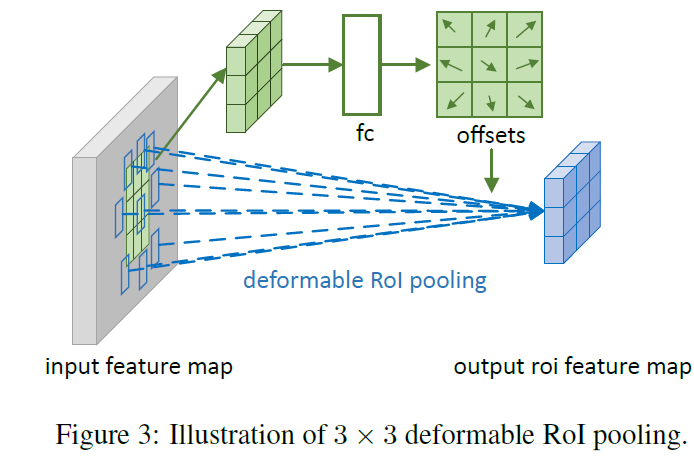
먼저 RoI pooling ( Eq 5 )는 pooled feature maps 를 생성하죠. maps로부터, fc layer는 normalized offset delta hat p_ij를 생성하죠. 그런 다음 Eq 6에서 offset delta p _ij 로 transformed 되죠 . 이는 RoI's width와 height를 가진 element-wise product 에 의해 transformed되죠. 식으로 표현하면 아래와 같습니다.
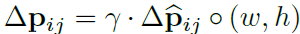
gamma는 pre-defined된 scalar 인데 offsets의 magnitude를 modulate하죠. 실험적으로 gamma = 1 로 set합니다. offset normalization은 offset learning을 RoI size에 invariant 하게 하기 위해 필요합니다. fc layer는 backpropagation에 의해 learned 됩니다.
Position-Sensitive (PS) RoI Pooling
이것은 fully convolutional로 RoI pooling과는 다르죠. conv layer를 통해, 모든 input feaure maps는 먼저 각 object class를 위한 k^2 score maps로 converted됩니다. 이는 Figure 4에서 bottom branch에 나타나 있죠.
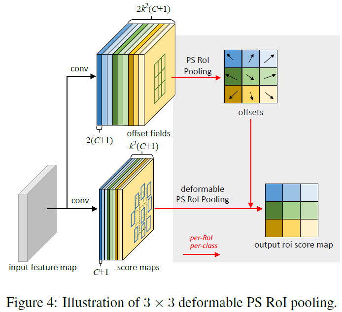
classes 간 distinguish할 필요 없이, such score map은 { x _i.j } 로 표기되죠. ( i , j )는 all bins를 나열하고요. pooling은 이 score maps에 수행됩니다. ( i, j )-th bin을 위한 output value 는 one score map x _ i, j 로 부터 그에 해당하는 bin 으로 summation 함으로써 obtained 되죠. 요약하면, Eq 5에서 RoI pooling과 다른점은 general feature map x 가 specific positive-sensitive score map x_i,j 에 의해 대체되어진다는 것이죠.
deformable PS RoI pooling에서, Eq 6에서의 변화는 x가 x_i,j로 바뀐다는 것이죠. 그러나, offset learning은 다릅니다. 이는 Figure 4에 설명된 것과 같죠. top branch에서, conv layer는 full spatial resolution offset fields를 생성합니다. 각 RoI에 대해, PS RoI pooling은 normalized offsets delta hat p _i,j를 obtain하는 such fields에 applied 되죠. 이는 그런다음 real offset delta p_i,j로 transformed되고 방식의 위에서 설명한 RoI pooling과 같습니다.
Deformable ConvNets
deformable convolution과 RoI pooling modules 모두 plain version과 같은 input과 output를 가집니다. 따라서 그들은 existing CNNs에서 their plain counterparts와 쉽게 replace 될 수 있죠. training 에서. offst learning을 위해 conv와 fc layers 가 추가된 이들은 zero weights로 initialized 됩니다. their learning rates는 existing layers에 대해 learning rate의 beta imes로 set되는데 beta = 1이 기본이고 Faster R-CNN에서 fclayer에 대해 beta = 0,01이죠. 그들은 back propagation을 통해 trained되는데 backporpagation은 Eq 3, 4 에서 bilinear interporation operation을 이용해 이뤄지죠. 이 resilting CNNs를 deformable ConvNets라고 부릅니다.
deformable ConvNets를 SOTA architectures와 integrate하기 위해, 먼저 이 architecture가 two stage로 구성되어 있음을 알립니다. 먼저, deep fully convolutional network는 whole input image에 걸처 feature maps를 generates하고 shallow task specific network가 feature map으로부터 results를 generate하죠.
Deformable Convolution for Feature Extraction
저자들은 feature extraction을 위한 two SOTA architecture에 adpot 하죠: ResNet 101 과 InCeption-ResNet의 modifed version 이죠. 둘 모두 imageNet classification dataset에 대해 pre-trained 되었죠.
original Inception-ResNet은 image recognition을 위해 designed 되었죠. inception-resnet은 feature misalignment issue와 dense prediction tasks에 대해 problematic을 가지고 있죠. modified version은 "Aligned-Inception-ResNet" 으로 불립니다.
두 models는 several convolutional blocks, average pooling 그리고 ImageNet classification을 위한 1000-way fc layer로 구성되어 있죠. average pooling과 fc layers는 제거되죠. randomly initialized 1 x 1 convolution은 channel dimension을 1024로 reduce 하기 위해 마지막에 추가됩니다. 일반적 관례와 같이, last convolutional block에서 effective stride는 32 pixcels를 16pixels로 feature map resolution을 increase하기 위해 reduced되죠. 구체적으로, last block의 begining에서 stride는 2에서 1로 바뀝니다. ( ResNet-101과 Aligned-Inception-ResNet에서 " conv 5 " ). compensate하기 위해, all convolution filters의 dilation이 1에서 2로 바뀌고요. 물론 kerner size가 1보다 큰 block들에 대해서겠죠.
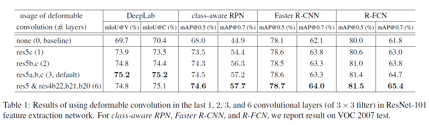
optionally하게, deformable convolution은 마지막 few convolutional layers에 applied됩니다. 저자들은 layers의 different numbers를 가지고 실험했고 3이 different tasks를 위한 good trade-off라는 것을 알아냈죠. 이는 Table 1에서 볼 수 있습니다.
Segmentation and Detection Networks
task specific network는 output feature mpas에 대해 built되는데 feature extraction network로 부터의 freature maps를 말하죠.
아래서, C는 object classes의 number를 표기합니다. DeepLab은 SOTA method 이고 semantic segmentation에 대한 network이죠. per-pixel classification scores를 represent하는 ( C + 1 ) maps를 생성하는 feautre map에 걸쳐 1 x 1 convolutional layer를 추가합니다. 따라나오는 softmax layer는 per-pixel probabilities를 outputs하죠.
Category-Aware RPN은 region proposal network과 거의 유사합니다. 2-class ( object or not ) convolutional classifier가 ( C + 1 ) - classconvolutional classifier로 대체 된것을 제외하면 말이죠. SSD의 simplified version으로도 볼 수 있죠.
Faster R-CNN은 SOTA detector 인데요. 저자들의 구현에서, RPN branch는 conv4 block의 위에 추가 됩니다. 기존 연구에서, RoI pooling layer는 ResNet-101에서 conv4와 conv5 blocks 사이에 insert되죠. 각 RoI 를 위해 10 개의 layers를 남겨놓습니다. 이 design은 좋은 성능을 보여줍니다만 높은 per-RoI computation을 가지죠. 대신에, 저자들은 simplifed design을 adopt합니다. RoI pooling layer가 마지막에 added되죠. pooled RoI features의 위에, 1024 dimension을 가지는 두 개의 fc layer를 추가합니다. 이는 bounindg box regression과 classification branches 뒤에 따라나오죠. such simplification이 accuracy를 감소시키지만, 여전히 strong enough baseline을 만들고, 이 연구에서 관심 대상이 아니죠.
optionally하게, RoI pooling layer는 deformable RoI pooling으로 바뀔 수 있습니다.
R-FCN은 또 다른 SOTA detector인데요. per-RoI computation cost를 무시할만 합니다. 저자들은 original implementation을 따르고 optionally하게 its RoI pooling layer는 deformable position-sensitive RoI pooling으로 바꿀 수 있습니다.
Understanding Deformable ConvNets
이 연구는 target tasks로부터 additional offsets와 learning offsets을 가지는 convolution과 RoI pooling에서 spatial sampling locations를 augmenting하는 것에 대한 idea에 대해 built됩니다.
deformable convolution이 stacked될 때, composited deformation의 effect는 profound한데요. 이 예시는 Figure 5에 나타나 있죠
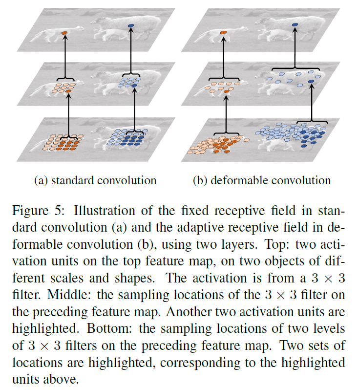
receptive field와 locations를 standard convolution에서 sampling하는 것은 top feature map( left )에 걸처 fixed됩니다. 그들은 adaptively하게 adjusted되는데 이는 deformable convolution에서 objects' scale과 shape에 따라서 행해지죠 ( right ). 더 많은 예시가 Figure 6에 나타나있죠.
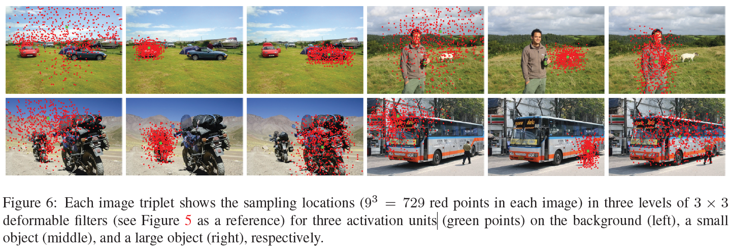
Table 2는 such adaptive deformation의 quantitative evidence를 제공하죠
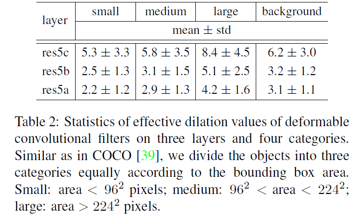
deformable RoI pooling의 effect는 유사하고 Figure 7에 나타나있습니다.
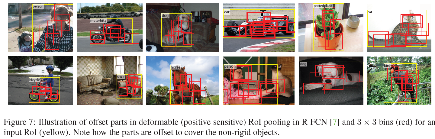
standard RoI pooling에서 gird structure의 regularity는 더 이상 쓸모가 없죠. 대신에, parts는 RoI bins로부터 deviate하여 nearby object foreground regions으로 옮겨가죠. localization capability 가 강화되죠. 특히 non-rigid object에 대해 말이죠.
In Context of Related Works
저자들의 연구는 previous works와 different aspests에서 관련이 있는데요. 저자들은 relations와 differences에 대해 자세히 설명한다고 합니다.
Spatial Transform Networks ( STN )
STN은 deep learning framework에서 data로부터 spatial transformation을 learn하는 첫 번째 연구였죠. 이는 global parametric transformation을 통해 feature map을 warp하죠. 가령 affine transformation이 있죠. 이런 warping은 expensive 하고 transformation parameters을 learning하는 것은 어렵다고 알려져있죠. STN은 small scale image classification problem에서 성공을 거뒀죠. inverse STN method는 expensive feature warping을 efficient transformation parameter propagation으로 대체합니다.
deformable convolution에서 offset learning 은 STN에서 extremely light-weight spatial transformer로 볼 수 있죠. 그러나 deformable convolution은 global parametric transformation과 feature warping을 adopt하지 않죠. 대신에, local하고 dense한 방식으로 feature map을 sample하죠. new feature maps를 generate 하기 위해, weighted summation step을 가지고 있는 이는 STN에서는 결여되어 있죠.
Deformable convolution은 any CNN architectures로 쉽게 integrate 하죠. desne ( e.g semantic segmentation ) 이나 semi-dense (e.g. object detection) predictions가 요구하는 complex vision tasks에 대해 effective하죠.
Active Convolution
이 연구는 contemporary합니다. 이 역시 offsets를 가진 convolution에서 sampling locations를 augment하고 back-propagation end-to-end를 통해 offsets를 learns하죠. 이는 image classification tasks에 대해 effective합니다.
deformable convolution과 crucial differences는 active convolution은 less general 하고 adaptive하다는 겁니다. 먼저, 그것은 offsets를 different spatial locations에 대해 공유합니다. 두 번째로, offsets는 per task나 per training에 의해 learnt되는 static model parameters이죠. 반면에, deformable convolution에서 offsets는 per image location을 다양하게 하는 dynamic model outputs이죠. 그들은 images에서 dense spatial transformations를 model하죠. 그리고 (semi-) dense prediction tasks에 효과적이죠.
Effective Receptive Field
이는 receptive field에서 all pixels가 output response에 동일하게 기여하는 것은 아니라는 사실을 발견합니다. center와 가까운 pixels가 훨씬 영향력이 있죠. effective receptive field는 theoretical receptive field의 small fraction 만을 차지합니다. 그리고 Gaussian distribution을 가지죠. 비록, theoretical receptive field size가 convolutional layers의 수에 따라 linearly하게 증가하지만, surprising result는 effective receptive field size는 square root의 수에 따라 linearly하게 증가한다는 것이죠. 그럼으로 우리가 생각하는 것보다 훨씬 천천히 증가하죠.
이 finding은 심지어 deep CNNs에서 top layer's unit 조차도 충분히 큰 receptive field를 가지지 못한다는 것을 나타냅니다. 이것은 부분적으로 atrous convolution이 vision task에서 왜 widely하게 쓰이는 지 설명합니다. 이는 adaptive receptive field learning이 필요성을 나타내죠.
Deformable convolution은 receptive fields를 adaptively하게 learning할 수 있죠.
Atrous convolution
atrous convolution은 normal filter's stride를 1보다 크게하여 sparsified sampling locations에서 original weights를 keeps합니다. 이( dilated convolution이라고 불리기도하는 이 convolution)는 receptive field size를 increase하고 parameters와 computation에서 same complexity를 retain하죠. 이는 semantic segmentation, object detection그리고 image classification에서 널리 사용되죠.
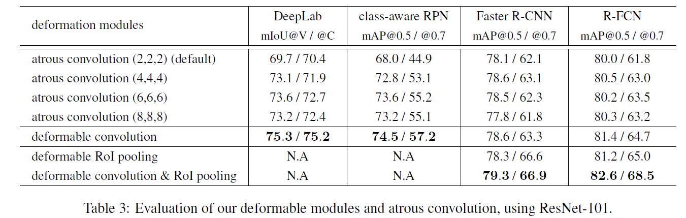
Deformable convolution은 atrous convolution의 generalization입니다. atrous convolution과 Extensive comparision은 Table 3에 나타나있죠.
Deformable Part Models ( DPM )
Deformable RoI pooling은 DPM과 유사하죠. 왜냐하면 둘 모두 classification score를 maximize하는 object parts의 spatial deformation을 learn하기 때문이죠. Deformabla RoI pooling은 더 simpler한데 parts 간에 spatial relations를 고려하지 않아도 되기 때문이죠.
DPM은 shallow model 인데 deformation을 modeling하는 capability를 제한하죠. its inference algorithm은 distance transform을 special pooling operation으로 다룸으로써 CNNs로 converted될수 있는 반면, its training은 end-to-end가 아니고 componets나 part sizes의 selection과 같은 heuristic choices가 포함되죠. 반면에, deformable ConvNets은 deep하고 end-to-end training을 수행하죠. multiple deformable modules가 stacked될 떄, deformation을 modeling하는 capability는 더 stronger해지죠.
DeepID-Net
DeepID-Net은 deformation constrained pooling layer를 도입하는데 이는 object detection을 위한 part defromation으로 consider합니다. 그럼으로 그것은 deformable RoI pooling과 유사한 정신을 공유하죠. 그러나 훨씬 복잡합니다.
이 연구는 RCNN에 기반하고 engineered 되었죠. 이것은 recent SOTA object detecttion methods를 end-to-end 방식으로 adapt하는 방법에 대해 unclear하죠.
Spatial manipulation in RoI pooling
spatial pyramid pooling은 hand crafted pooling regions을 scales에 걸쳐 사용하죠. 이는 predominant approach이고 deep learning based object detection에 사용되었죠.
pooling regions의 spatial layout을 learning하는 것에 대한 연구는 거의 없습니다. 한 연구는 large over-complete set으로 부터 pooling regions의 sparse subset에 대해 learns합니다. large set은 hand engineered 되었고 end-to-end 가 아니죠.
Deformable RoI pooling은 pooling regions를 CNNs에서 end-to-end로 learn하는 데에 선구자입니다. regions가 same size이긴 하지만, multiple size로 extension은 직관적이죠.
Transformation invariant Features and their learning
transformation invariant features를 designing하는데에 굉장히 많은 노력이 있었죠. SIFT, ORB 가 그 예이고요. CNNs의 context에서 이런 연구는 큰 부분을 차지하죠. image transformations에 대한 CNN representations의 equivalence와 invariance는 다른연구에 있습니다. 몇몇 연구는 invariant CNN representations에 대해 learn하는데 이는 transformations의 different type에 관한 연구였죠. scattering networks, convolutional jungles, TI pooling과 같은 것들이 있죠. 몇몇 연구는 specific transformations에 헌신했는데 symmetry, scale, rotation과 같은 specific transformation에 관한 것이었죠.
위에 언급된 연구들에서 transformations는 priori로 알려져 있죠. knowledge는 CNNs 기반한 learnable parameters를 가지고 feature extraction algorithm의 structure를 hand craft하는데 사용되었고요. 그들은 unknown transformations를 handle할 수 없죠.
반면에, deformable modules는 various transformations에 generalize합니다. transformation invariance는 target task로 부터 learned되죠.
Dynamic Filter
deformable convolution과 유사하게, dynamic filters는 input feature에 대해 conditioned되고 samples에 걸쳐 변합니다. 다른점은, filter weights만 learned된다는 것이죠. 이 연구는 video와 stero prediction에 applied됩니다.
Combination of low level filters
Gaussian filters나 its smooth derivatives는 low level image structures를 extract하는데 널리 사용되죠. low level image structures에는 corners, edges, T-junctions등이 있죠. 특정 conditions에서 , such filters는 basis의 set을 form하고 their linear combination은 greometric transformations의 같은 group안에서 new filters를 forms하죠. multiple orientations in steerable Filters 가 예가 되겠네요.
deformable kernels가 다른 연구에서 사용되긴 했지만, its meaning은 저자들의 연구에서와는 다르다고합니다.
Most CNNs는 scratch 로 부터 all their convolution filters를 learn합니다. 최근 연구는 이는 필요 없을 수도 있ㄷ는 것을 보여주고요. 이는 low level filters의 weighted combination에 의해 free form filters를 replace합니다. 그리고 weight coefficients를 learn하죠. filter function space에 걸친 regularization은 training data가 작을 때 generalization ability를 향상시킴을 보여줬죠
위의 연구는 저자들의 연구와 관련됩니다. different scale을 가진 multiple filters가 combined될 때 resulting filter는 complex weights를 가질수 있고 deformable convolution filter를 resemble하죠, 그러나, deformable convolution은 filter weights 대신에 sampling locations를 learn합니다.
오늘도 실험파트는 생략합니다.
뭔가 길었어요 내용이 ㅎㅎ 그럼 다음에뵈요


