안녕하세요. WH입니다.
RAFT 라는 모델에 대한 opticalflow estimation model인데요
2022 기준 SOTA 모델은
RAFT의 변형이 많기에 토대를 이루는 논문을
읽어보도록할게요
Abstract
저자들은 Recurrent All-Pairs Field Transforms (RAFT)를 도입합니다. 이는 optical flow를 위한 새로운 deep network architecture죠. RAFT는 per-pixel features를 추출하고 pixels의 all pairs에 대한 multi-scale 4D correlation volumes를 만들죠. 그리고 반복적으로 flow field를 recurrent unit을 통해 업데이트하는데, 이 unit은 correlation voulmes에 대한 lookups를 수행하죠. RAFT는 ( 20년 기준 ) SOTA를 달성했죠.
Introduction
Optical flow는 video frames 간의 per-pixel motion을 estimating하는 task 인데요. 이는 해결되지 않은 오래된 vision problem이죠. best system은 fast-moving objects, occlusions, motion blur, 그리고 textureless surfaces를 포함하는 문제에 의해 제한되죠.
Optical flow는 전통적으로 한 쌍의 이미지 간의 dense displacement fields 에 대한 hand-crafted optimization problem으로 접근되어 왔는데요. 일반적으로 optimization objective는 시각적으로 유사한 이미지 regions의 alignment를 encourage하는 data term과 motion의 타당성에 대해 우선권을 부여하는 regularization term 간의 trade-off를 정의하죠. 이런 approach는 상당한 성공을 이뤄냈죠. 그러나, 더 나아가 progress 는 challenging했죠. corner cases의 variety에 robust한 optimization objective를 hand-designing하는것이 어렵기 때문이죠.
최근, deep learning은 traditional methods에 대한 유망한 대안으로 보여졌죠. Deep learning은 optimization problem에 대한 formulating을 보조적으로 수행할 수 있고 flow를 직접적으로 예측하는 network를 훈련할 수 있죠. Current deep learning methods는 traditional methods와 견줄만한 성능을 달성했죠. inference time은 훨씬 빠르고요. 앞으로의 연구를 위한 key question은 성능이 더 잘나오고, 학습이 쉬우며, 새로운 scenes에 일반화하는 effective architecture를 designing하냐죠.
저자들은 RAFT를 도입하죠. 새로운 deep network architecture이고 optical flow를 위한 모델입니다. RAFT는 다음의 장점을 지니고 있죠.
1. SOTA accuracy
2. Strong generalization
3. High efficiency ( 지금은 해당하지 않는 말이긴 합니다 )
RAFT는 3개의 main components로 구성되어있죠. (1) each pixel에 대한 feature vector를 추출하는 feature encoder (2) lower resolution volumes를 생성하는 subsequent pooling을 가진 pixels의 all pairs에 대한 4D correlation volume을 생성하는 correlation layer (3) correlation volumes로 부터 value를 retrieve하고 0으로 초기화된 flow field를 반복적으로 update하는 recurrent GRU-based update operator. 이는 Fig.1 에 설명된 RAFT design에서 볼 수 있죠

RAFT architecture는 traditional optimization-based approaches에 영감을 받았는데요. feature encoder는 per-pixel features를 추출하죠. correlation layer는 visual similarity를 pixels 간에 계산합니다. update operator는 iterative optimization algorithm의 steps를 모방합니다. 그러나, traditional approaches와 다르게, features와 motion priors는 handcrafted 가 아니고 learned죠. feature encoder와 update operator에 의해 learned되죠.
RAFT의 design은 많은 연구로부터 영감을 반영했는데요. 상당히 새로운 architecture죠. 먼저, RAFT는 high resolution에 single fixed flow field를 updates하고 maintains하죠. 이는 이전 연구의 prevailing coarse-to-fine design과는 상당히 다르죠. 여기서 flow는 먼저 low resolution에서 estimated되고 high resolution에서 resampled와 refined 되죠. single high-resolution flow field에 대해 operating 됨으로써, RAFT는 coarse-to-fine cascade의 한계를 극복했죠. coarse resolutions에서 error로부터 recovering하는 것에 대한 어려움, small fast-moving objects를 놓치는 경향, 그리고 multi-stage cascade를 training에 대해 여구하는 많은 training iterations 와 같은 한계를 극복했습니다.
두 번째로, RAFT의 update operator는 recurrent 하고 lightweight합니다. 많은 최근 연구는 iterative refinement의 몇몇 형태를 포함하는데요. iterations에 걸쳐 weights를 tie하지 않죠. 그렇기 때문에 fixed number of iterations에 한계를 지녔고요. 자신들이 아는 범위내에서, IRR만이 recurrent한 deep learning approach 죠. FlowNetS 나 PWC-Net을 recurrent unit으로 사용했고요. FlowNetS를 사용했을 때, network size에 한계를 지녔기에, 5 번의 iterations까지만 적용되었죠. PWC-Net을 사용했은때는, pyramid levels의 수에 제한을 받았습니다. 반면에, RAFT는 update operator를 100+ 이상 inferece 동안 divergence 없이 적용할 수 있죠.
세 번째, update operator는 새로운 design인데요, convolutional GRU로 구성되어 있죠. convolutional GRU는 4D multi-scale correlation volumes에 대해 lookups를 수행합니다. 반면에, prior work에서 refinement modules은 오직 plain convolution이나 correlation layers를 사용했죠.
저자들은 Sintel 과 KITTI에서 실험을 진행했고 SOTA 성능을 달성했다고 합니다.
Related Work
Optical Flow as Energy Minimization
Optical flow는 전통적으로 energy minimization problem으로 다뤄졌는데요. data term과 regularization term의 trade-off 관계를 부과하죠. Horn과 Schnunck은 optical flow를 continuous optimizaition problem으로 공식화 했는데요 variational framework를 사용했죠. 그리고 dense flow field를 gradient steps을 수행함으로써 추정할 수 있었죠. Black 과 Anandan은 oversmoothing과 noise sensitivity를 가진 문제로 다뤘죠. robust estimation framework을 도입했고요. TV-L1은 L1 data term과 total variation regularization을 가진 quadratic penalties 대체했습니다. 이는 motion discontinuities를 허용하고 outliers를 더 잘 다루도록 해주었죠. Improvements는 matching costs와 regularization terms를 더 잘 defining함으로써 이뤄졌습니다.
이런 continuous formulations는 optical flow의 singe estimate를 maintain하죠. 각 iteration에서 refined되고요. smooth objective function을 ensure하기 위해, first order Taylor approximation이 data term을 model하는데 사용됩니다. 결과적으로, 그들은 small displacements에서만 잘 작동하죠 ( 왜냐면 large displacement는 선형과는 오차가 크기 때문이죠 여튼) large displacements를 다루기 위해, coarse-to-fine strategy 가 사용되었습니다. 여기서 image pyramid는 low resolution 에서 large displacements를 추정하는 데 사용되죠. 그 뒤에, small displacements가 high resolution에서 refined되죠. 그러나 이 coarse-to-fine strategy는 small fast-moving objects를 놓칠지도 모르고 early mistakes로부터 recovering하는데에 어려움이 있죠. continuous methods와 유사하게, 저자들은 optical flow의 single estimate을 maintain합니다. 즉 each iteration마다 refined하죠. 그러나, 저자들이 low resolution과 high resolution 모두에서 all pairs에 대해 correlation volumes를 build하기 때문에, 각 local update는 small 과 large displacements 모두에 대한 정보를 사용합니다. 게다가, data term의 subpixel Taylor approximation을 사용하는 것 대신에, update operator는 descent direction을 propose하기 위해 학습합니다.
최근에, optical flow는 discrete optimization problem으로써 접근되어왔는데요. 이 approach의 하나의 challenge는 search space의 massive size입니다. each pixel이 다른 frame에서 수 천개의 points와 paired 되기 때문에 발생하죠. Menez et al은 search space를 feature descripotrs를 사용해 pruned하고 message passing을 사용해 global MAP estimate를 approximated합니다. Chen et al은 distance transform을 사용함을써, flow fields의 full space에 걸쳐 globel optimization problem을 해결하는 것이 tractable하다는 것을 보여줍니다. DCFlow는 feature descriptor로써 neural network를 사용함으로써 성능향상을 보여줬습니다. 그리고 4D cost volume을 features의 allparis에 대해 constructed했죠. 4D cost volume은 Semi-Global Matching algorithm을 사용해 처리되죠. DCFlow와 비슷하게, 저자들은 4D cost volumes를 학습된 features에 대해 constructed 하죠. 그러나 SGM을 사용해 cost volumes를 processing하는 대신에, 저자들은 flow를 추정하는 neural network를 사용하죠. 저자들은 approach는 end-to-end differentiable합니다. feature encoder가 의미하는 것은 final flow estimate의 error를 최소하는 network의 rest를 학습하는 것이라 할 수 있죠. 반면에, DCFlow는 pixels 간의 embedding loss를 사용하여 학습됩니다. optical flow에 대해 직접적으로 학습될 수 없죠. 왜냐하면 cost volume processing이 differentiable하지 않기 때문이죠.
Direct Flow Prediction
NN은 frames간에 optical flow를 직접적으로 예측하기 위해 학습될 수 있죠. optimization problem을 보조적으로 수행하고요. Coase-to-fine processing은 많은 연구에서 popular ingredient로써 떠올랐는데요. 반면에 저자들의 방법은 single high-resolution flow field를 maintains하고 updates하죠.
Iterative Refinement for Optical Flow
많은 연구가 optical flow에 대해 results를 improve하는 iterative refinement를 사용하죠. Ilg et al은 optical flow에 iterative refinement를 적용했는데요. multiple FlowNetS와 FlowNetC modules를 일렬로 쌓았죠. SpyNet, PWC-Net, LiteFlowNet 긔고 VCN은 iterative refinement를 적용했는데 coarse-to-fine pyramids를 사용했죠. 이 approaches과의 차이는 이 방법들은 itertions 간에 weights를 share하지 않는다는 것이죠.
우리 approach와 가까운 approach는 IRR인데요. IRR은 FlownetS 와 PWC-Net을 기반으로 구축되었죠. 그러나 refinement networks 간에 weights를 share하죠. FlowNetS를 사용할때, network의 size에 의해 제한됩니다. 따라서 5 번의 iterations까지만 적용될 수 있습니다. PWC-Net을 사용하면 pyramid levels에 수 에 의해 제한됩니다. 반면에, 저자들은 simpler refinement module을 사용하고 100+ 의 iterations를 적용할 수 있죠. 저자들의 방법은 Devon을 활용한 similarites를 share합니다. wraping과 fixed resolution updates 없는 cost volume의 construction이죠. 그러나, Devon은 recurrent unit이 없죠. large displacement에 대해 저자들의 것과 차이가 있습니다. Devon은 large displacements를 dilated cost volume을 사용해 다루는 반면 저자들의 approach는 multiple resolutions에서 correlation volume을 pools 합니다.
저자들의 방법은 TrellisNet과 Deep Equilibrium Models와 관련이 있는데요. TrellisNet은 많은 layer에 weights가 tied된 depth를 사용하고 DEQ는 많은 layer를 simulates합니다. fixed point를 직접 solving함으로써 말이죠. TrellisNet과 DEQ는 sequence modling tasks를 위해 designed 되었습니다. 그러나 저자들은 weight-tied units의 많은 수를 사용하는 core idea를 적용합니다. 저자들의 update operator는 modified GRU block을 사용합니다. LSTM block과 비슷한데 이는 TrellisNet에 사용되었죠. 저자들은 이 structure가 자신들의 update operator를 더 쉽게 fixed flow field로 수렴하도록 한다는 것을 알게 되었다고 합니다.
Learning to Optimize
많은 problems는 optimization problem으로 formulated될 수 있죠. 이는 optimization problem을 network architectur로 embed하는 연구에서 motivated되었죠. 이 연구들은 전형적으로 inputs나 optimization problem의 parameters 예측하는 network를 사용합니다. 그리고나서 network weights를 학습하죠. solver를 통해 gradient를 backpropogating하는 방식으로요. 그러나 이 technique은 쉽게 정의된 objective를 가진 problem에 한계가 있죠.
또 다른 approach는 data로부터 iterative updates를 학습하는 것입니다. 이 approaches는 first order optimizer는 iterative update steps의 sequence로써 표현될수 있다는 사실에서 motivated됩니다. Adler et al는 optimizer를 직접 사용하는 대신에, first order algorithm의 updates를 모방한 network를 building할 것을 제안하죠. 이 approach는 inverse problems에 적용되었습니다. inverse problem에는 image denoising, tomographic reconstruction그리고 novel view synthesis가 있죠. TVNet은 TV-L1 algorithm을 computation graph로 구현했습니다. TV-L1 parameters를 학습할 수 있게 해주죠. 그러나 TVNet은 learned features 대신 intensity gradients에 기반해 연산하죠. 이는 Sintel과 같은 dataset에서 accuracy에 큰 문제가 있죠.
저자들의 approach는 optimize하는 learning으로써 볼 수 있습니다. 저자들의 network은 수 많은 update blocks를 사용하죠. 이 block은 first-order optimization algorithm의 step을 emulate하고요. 그러나 기존 연구와 다르게, 저자들은 optimization objective에 관한 gradient를 명확하게 define하지 않습니다. 대신에, 저자들의 network가 descent direction을 제안하는 correlation bolumes으로 부터 features를 retrieves하죠.
Approach
consecutive RGB images의 쌍이 주어지면, I_1, I_2 , 저자들은 dense displacement field( f^1, f^2 )를 추정합니다. 이 field는 I_2에서 each pixel ( u, v )를 I_2에서 그것에 corresponding coordinates로 maps하죠 즉 식으로 표현하면 아래와 같습니다.

저자들의 approch의 overview는 Fig1에 주어져있죠. 저자들의 method는 3 개의 단계로 distilled 될 수 있습니다. (1) feature extraction, (2) computing visual similarity, 그리고 (3) iterative updates. 여기서 모든 stages는 differentiable하고 end-to-end trainable architecuture로 구성될 수 있습니다.
Feature Extraction
Features는 input images로 부터 convolutional network를 사용해서 추출됩니다. Feature encoder network는 I_1 과 I_2 모두에 적용됩니다. 그리고 input images를 dense feature maps에 lower resolution에서 map 합니다. 저자들의 encoder는, g_thetha 는 1/8 resolution에서 features를 outputs합니다.

여기서 D = 256으로 set했습니다. feature encoder는 6 개의 residual blocks로 구성되어 있습니다. 1/2, 1/4, 1/8 resolution에서 각각 2개가 있죠.
저자들은 추가적으로 context network을 사용합니다. context network는 I_1 image에서만 features를 extract하죠. h_thetha 는 feature extraction network와 동일합니다. 둘 모두는 한번만 수행되고, first stage에서 만들어집니다.
Computing Visual Similarity
저자들은 visual similarity를 all pairs 간의 full correlation volume을 constructing 함으로써 계산하죠. image feature g(I_1), g(I_2) 가 주어지면, correlation volume은 feature vectors의 all paris 간에 dot product를 수행하여 얻어지죠. correlation volume, C , 는 single matrix multiplication으로써 효율적으로 계산될 수 있습니다.

Correlation Pyramid
저자들은 4-layer pyramid { C^1, C^2, C^3, C^4 }를 construct하죠. 이는 kernel sizes 1, 2, 4, 8과 equivalent stride을 가진 correlation volume의 last two dimensions를 pooling함으로써 construct합니다. 이는 Fig 2.에 나와 있죠.

따라서, volume C^k는 H x W x H/2^k x W/2^k 의 dimensions를 가집니다. volumes의 set은 large 와 small displacements 모두에 대한 information을 주죠. 그러나, 처음 2 dimension을 maintaining함으로써 저자들은 high resolution information을 maintain 하고 이는 저자들의 방식이 small fast-moving objects의 motions를 recover 하게 해주죠.
Correlation Lookup
lookup operator를 L_C라고 정의합니다. L_C는 feature map을 생성하는데 correlation pyramid로부터 indexing하는 방식으로 생성하죠. optical flow의 current estimate ( f^1, f^2 )가 주어지면, 저자들은 I_1의 each pixel x = ( u, v )을 I_2의 estimated correspondence로 map합니다. 식으로 보면 아래와 같죠

저자들은 그러고 난 뒤 x' 주위에 local grid를 정의합니다

integer offsets의 set은 x' 의 radius r 안에서 존재하며 L1 distance를 사용합니다. 저자들은 local neighborhod N(x')_r 을 사용하는데 local neighborhood는 correlation volume으로부터 index하죠. N(x')_r 이 real numbers의 grid이기 때문에, 저자들은 bilinear sampling을 사용합니다.
저자들은 lookups를 pyramid의 모든 levels에 대해 수행합니다. 그렇게 함으로써 level k에서 correlation volume , C^k, 는 grid N(x'/2^k)_r을 사용하여 indexed되죠. levels에 따른 constant radius는 lower level에서 larger context를 의미합니다. 가장 낮은 level에서, k = 4이고, original reolution에서 256 pixels의 range에 해당하는 radius 4를 사용하죠. 각 level로부터 values는 single feature map으로 concatenated 됩니다.
Efficient Computation for High Resolution Images
all pairs correlation scales O(N^2) 에서 N은 pixcels의 수 입니다. 이 scales는 한번만 계산됩니다. 그리고 iterations M의 numbers는 constant하죠. 그러나, 저자들의 approach의 equivalent implementation이 존재하는데요. inner product의 linearity와 average pooling을 사용하는 O ( N M )을 scales하는 것이죠. 이를 식으로 표현해보면 아래와 같습니다

m은 level을 뜻합니다. 2^m x 2^m grid에서 correlation response에 대한 average를 뜻하죠. 위 식은 C^m_ijkl에서 value가 feature vector g(I_1)_ij 와 2^m x 2^m size kernel을 가지고 pooled 한 g(I_2) 간에 inner product로써 계산되어진다는 것을 의미하죠.
이 alternative implementation에서 저자들은 correlations를 precompute 하지 않습니다. 대신 pooled feature maps를 precompute하죠. 각 iteration에서 저자들은 각 correlation value를 필요에 따라 compute 합니다. complexity는 O ( N M )이 되죠.
저자들은 실험적으로 all pairs를 precomputing하는 것이 impelment하기 쉽고 bottleneck이 아니라는 것을 알아냈다고 합니다. GPU 덕분이죠. 저자들은 alternative implementation으로 always switch 하는 것이 bottleneck이 될 수 있다는 것을 말해주네요.
Iterative Updates
update operator는 initial starting point f_0 = 0 로부터 { f_1, .... , f_N } flow estimates의 sequence를 estimate합니다. 각 iteration에서, update operator는 update direction delta f를 생성하는데요. current estimate에 적용되죠.

update operator는 flow, correlation, 그리고 latent hidden state을 input을 입력받고, update delta f와 updated hidden state을 outputs하죠. update operator의 architecture는 optimization algorithm의 steps를 mimic합니다. 그렇게 함으로써, 저자들은 depth에 걸쳐 tied weights를 사용합니다. 그리고 fixed point로 convergence를 encourage하는 bounded activations를 사용하죠. update operator는 updates를 수행하기 위해 학습되어지고 그렇게함으로써 sequence가 fixed point로 converge하죠.

Initialization
default로, 저자들은 flow field를 0으로 initialize합니다. 그러나 저자들의 iterative approach는 alternative를 활용한 실험에서 flexibility를 제공합니다. video에 적용할 떄, warm-start initialization을 test했죠. optical flow는 이전 frames의 쌍으로 만들어지고 다음 frames 쌍에 projected되죠. occlusion gaps는 nearest neighbor interpolation을 사용해 채워지고요
Input
current flow estimation f^k 가 주어지면, 저자들은 correlation features를 correlation pyramid로 부터 retirieve하는데에 사용합니다. Correlation features는 그러고 난 뒤 2 convolutional layers에 의해 처리되죠. 추가적으로 저자들은 2 convolutional layers를 flow features를 생성하는 flow estimate에 적용합니다. 마지막으로, 저자들은 직접 input을 context network로부터 inject하죠. input feature map은 correlation, flow, 그리고 context features의 concatenation으로 받아들여집니다.
Update
update operator의 core component는 gated activation unit인데요 GRU cell에 기반하죠. convolutions로 대체된 FC layers에 사용되는 GRU를 말합니다.
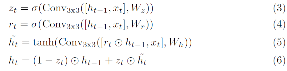
여기서 x_t는 flow, correlation, context features의 concatenation입니다. 저자들은 separable ConvGRU unit으로 실험을 했는데, 2 개의 GRU를 가진 3 x 3 convolution으로 대체했죠. 하나는 1 x 5 convolution 과 5 x 1 convolution을 사용했는데, receptive field를 model size의 증가 없이 증가시켰죠.
Flow Prediction
GRU에 의해 outputted되는 hidden state는 flow update delta f를 예측하는 두 개의 convolutional layers를 통과하는 데요. output flow는 1/8 resolution 입니다. training과 evaluation 동안, 저자들은 ground truth의 resolution과 match하는 predicted flow fields를 upsample합니다.
Upsampling
network outputs는 optical flow를 1/8 resolution에서 output합니다. 저자들은 optical flow를 full resolution으로 upsample합니다. each pixel에서 full resolution flow가 coarse resolution neighbors의 3x3 grid의 convex combination이 되도록 함으로써 말이죠. 저자들은 H/8 x W/8 x ( 8 x 8 x 9 ) mask를 예측하는 두 개의 convolutional layers를 사용합니다. 그리고 9 개의 neighbors의 weights에 대해 softmax를 수행하죠. final high resolution flow field는 neighborhood에 weighted combination을 취한 mask를 사용하고 그러고나서 Permuting 하고 H x W x 2 dimensional flow field로 reshaping함으로써 찾아지죠. 이 layer는 unfold function을 사용하면 pytorch에서 직접 구현가능합니다.
Supervision
저자들은 자신들의 network를 predicted와 ground truth flow 간 predictions의 full sequence에 대해 l_1 distance를 supervised 했습니다. ground truth flow f_gt가 주어지면 loss는 아래와 같이 정의 되고 감마는 0.8로 set했다고 합니다.

여기까지 하겠습니다.
PWC 지원안하는 하드웨어에서 돌리겠다고..
network를 다 뜯어고쳐가지고..
사실 pwc도 아니게 됬지만 여튼
고생좀했네요. 만족할 만한 결과는 아니지만
쓸만은 한데 역시나 욕심이 좀 나네요.
오늘은 여튼 여기까지 하겠습니다.


